Supervised Learning-Classification

July 4, 2023

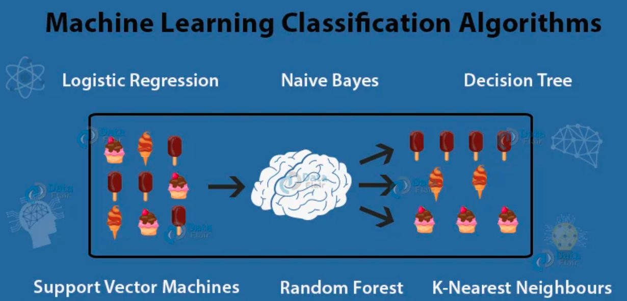
Classification is one of the most important aspects of supervised learning.

Logistic Regression

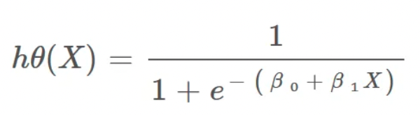
Logistic Regression is a Machine Learning algorithm that is used for classification problems.

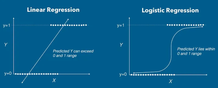
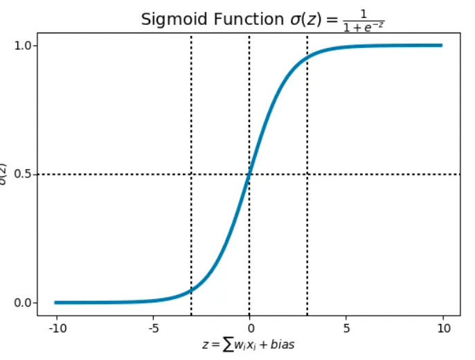
The hypothesis of logistic regression tends to limit the cost function between 0 and 1.

Decision Boundary

We have 2 classes, let’s take them like cats and dogs(1 — dog, 0 — cats). We basically decide with a threshold value above which we classify values into Class 1, and if the value goes below the threshold, then we classify it in Class 2.
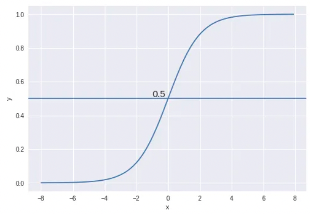
As shown in the above graph we have chosen the threshold as 0.5, if the prediction function returned a value of 0.7 then we would classify this observation as Class 1(DOG). If our prediction returned a value of 0.2 then we would classify the observation as Class 2(CAT).

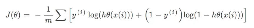
Cost Function

We learned about the cost function J(θ) in Linear regression*](https://towardsdatascience.com/introduction-to-linear-regression-and-polynomial-regression-f8adc96f31cb), the cost function represents the optimization objective, i.e. we create a cost function and minimize it so that we can develop an accurate model with minimum error.
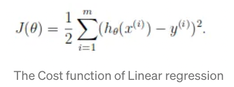
- If we try to use the cost function of the linear regression in ‘Logistic Regression’ then it would be of no use as it would end up being a non-convex function with many local minimums, in which it would be very difficult to minimize the cost value and find the global minimum.

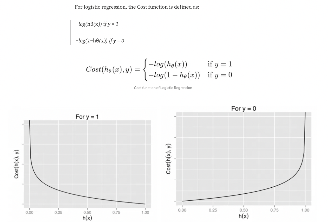
The above two functions can be compressed into a single function i.e.

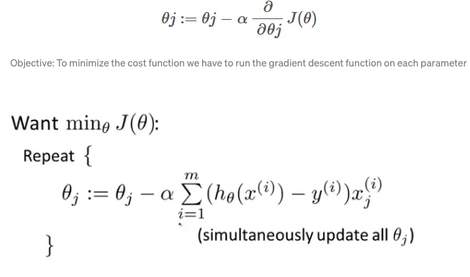
Gradient Descent

Now the question arises, how do we reduce the cost value? Well, this can be done by using Gradient Descent. The main goal of Gradient descent is to minimize the cost value. i.e. min J(*θ*).

Now to minimize our cost function, we need to run the gradient descent function on each parameter i.e.

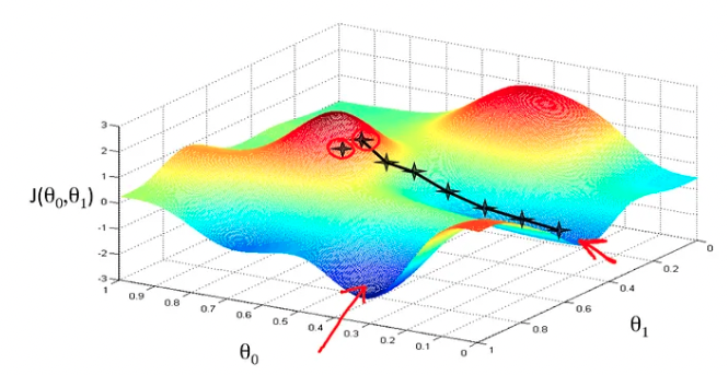
Gradient descent has an analogy in which we have to imagine ourselves at the top of a mountain valley and left stranded and blindfolded, our objective is to reach the bottom of the hill. Feeling the slope of the terrain around you is what everyone would do. Well, this action is analogous to calculating the gradient descent, and taking a step is analogous to one iteration of the update to the parameters.

Logistic Regression_Reference

Fisher’s Linear Discriminant

Background

Consider the binary classification (K=2)—blue and red points in R². Here, D represents the original input dimensions while D’ is the projected space dimensions. Throughout this article, consider D’ less than D. In the case of projecting to one dimension (the number line), i.e., D’=1, we can pick a threshold t to separate the classes in the new space.

We want to reduce the original data dimensions from D=2 to D’=1.
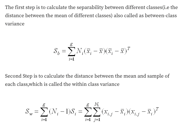
First, compute the mean vectors m1 and m2 for the two classes.

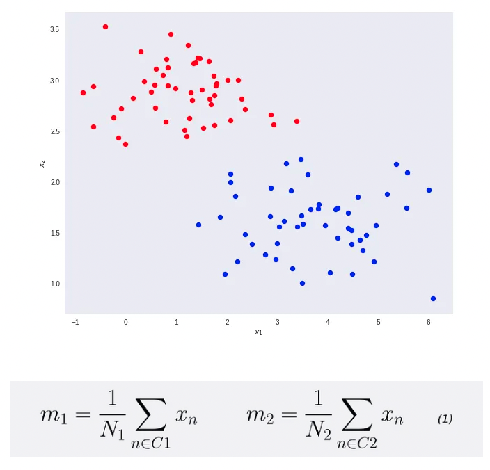
Note that N1 and N2 denote the number of points in classes C1 and C2, respectively.
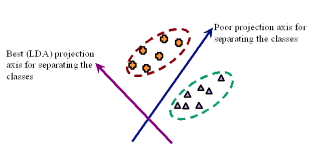
Now, consider using the class means as a measure of separation. In other words, we want to project the data onto the vector W joining the 2 class means.
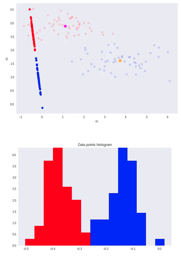
In this scenario, note that the two classes are clearly separable (by a line) in their original space.
However, after re-projection, the data exhibit some sort of class overlapping — shown by the yellow ellipse on the plot and the histogram below.

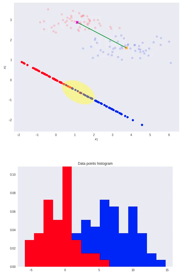
That is where Fisher’s Linear Discriminant comes into play.

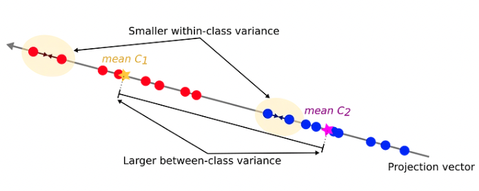
The idea proposed by Fisher is to maximize a function that will give a large separation between the projected class means while also giving a small variance within each class, thereby minimizing the class overlap.
In other words, FLD selects a projection that maximizes class separation. To do that, it maximizes the ratio between the between-class variance to the within-class variance.
A large variance among the dataset classes./ A small variance within each of the dataset classes.

To find the projection with the following properties, FLD learns a weight vector W with the following criterion.

Construct the lower dimensional space, which maximizes the between-class variance and minimizes the within-class variance.
Let W be the lower dimensional space projection, which is called Fisher’s criterion.

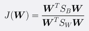
where

FDA for Multiple Classes

We can generalize FLD for the case of more than K>2 classes. Here, we need generalization forms for the within-class and between-class covariance matrices.

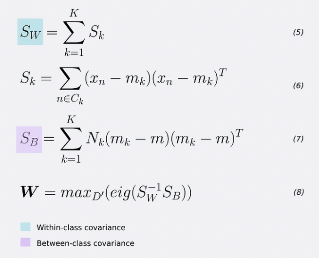
To find the weight vector W, we take the D’ eigenvectors that correspond to their largest eigenvalues (equation 8).
In other words, if we want to reduce our data dimensions from D=784 to D’=2, the transformation vector W is composed of the 2 eigenvectors that correspond to the D’=2 largest eigenvalues. This gives a final shape of W = (N,D’), where N is the number of input records and D’ the reduced feature space dimensions.

Building a linear discriminant

Up until this point, we used Fisher’s Linear discriminant only as a method for dimensionality reduction. To really create a discriminant, we can model a multivariate Gaussian distribution over a D-dimensional input vector x for each class K as:

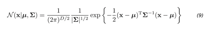
Here *μ* (the mean) is a D-dimensional vector. Σ (sigma) is a DxD matrix — the covariance matrix. And

is the determinant of the covariance. The determinant is a measure of how much the covariance matrix Σ stretches or shrinks space.

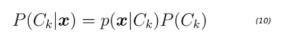
For multiclass data, we can (1) model a class conditional distribution using a Gaussian. (2) Find the prior class probabilities P(Ck), and (3) use Bayes to find the posterior class probabilities *p(Ck

x)*.

The parameters of the Gaussian distribution: μ* and Σ, are computed for each class k=1,2,3,…, K using the projected input data. We can infer the priors *P(Ck) class probabilities using the fractions of the training set data points in each of the classes (line 11).

Once we have the Gaussian parameters and priors, we can compute class-conditional densities P(x*

Ck)* for each class k=1,2,3,…, K individually. To do it, we first project the D-dimensional input vector x to a new D’ space. Keep in mind that D’ < D. Then, we evaluate equation 9 for each projected point. Finally, we can get the posterior class probabilities *P(Ck

**x*) for each class k=1,2,3,…, K using equation 10.

What are the steps in Linear Discriminant Analysis (LDA)?

Calculate the mean for each class and the overall mean
Calculate the within-class covariance matrix
Calculate the between-class covariance matrix
Calculate the eigenvalues and eigenvectors of the covariance matrices
Determine the linear discrimination functions
Construct a decision surface

Conclusion

LDA supports both binary and multi-class classification. It can be used for both binary and multiclass problems as well as to effectively shrink the number of features in the model.
LDA inherits the problems of GLM. It assumes the Gaussian distribution of the input variables. Always consider reviewing the univariate distributions of each attribute and using transforms to make them more Gaussian-looking.
Like GLM, outliers will affect the mean. Also, skew and kurtosis need to be checked for as they affect standard deviation.
Features assume that each input variable has the same variance.
It will help standardize the features and limit the standard deviation between 0 and 1.

SVM

Find the ideal hyperplane that differentiates between the two classes.
These support vectors are the coordinate representations of individual observation. It is a frontier method for segregating the two classes.
Based on these support vectors, the algorithm tries to find the best hyperplane that separates the classes.

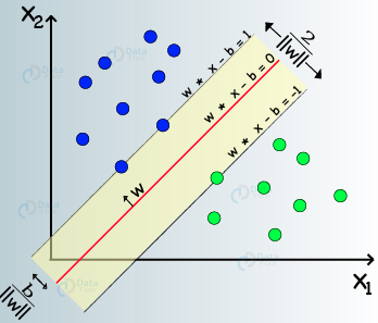
Intuitively the best line is the line that is far away from both apple and lemon examples (has the largest margin). To have an optimal solution, we have to maximize the margin in both ways (if we have multiple classes, then we have to maximize it considering each of the classes).

select two hyperplanes (in 2D) that separates the data with no points between them (red lines)
maximize their distance (the margin)
the average line (here the line halfway between the two red lines) will be the decision boundary

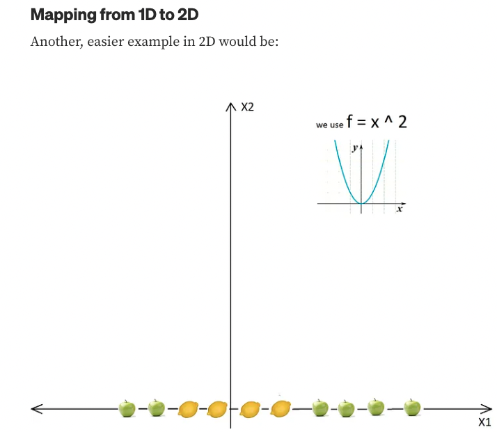
SVM for Non-Linear Data Sets

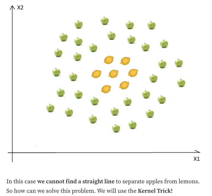
The basic idea is that when a data set is inseparable from the current dimensions, add another dimension, maybe that way, the data will be separable.
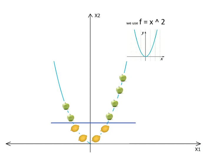
- Just think about it, the example above is in 2D, and it is inseparable, but maybe in 3D, there is a gap between the apples and the lemons. In this case, we can easily draw a separating hyperplane (in 3D a hyperplane is a plane) between levels 1 and 2.
- We just used a transformation in which we added levels based on distance.
- These transformations are called kernels. Popular kernels are Polynomial Kernel, Gaussian Kernel, Radial Basis Function (RBF), Laplace RBF Kernel, Sigmoid Kernel, Anove RBF Kernel, etc (see Kernel Functions or a more detailed description Machine Learning Kernels).
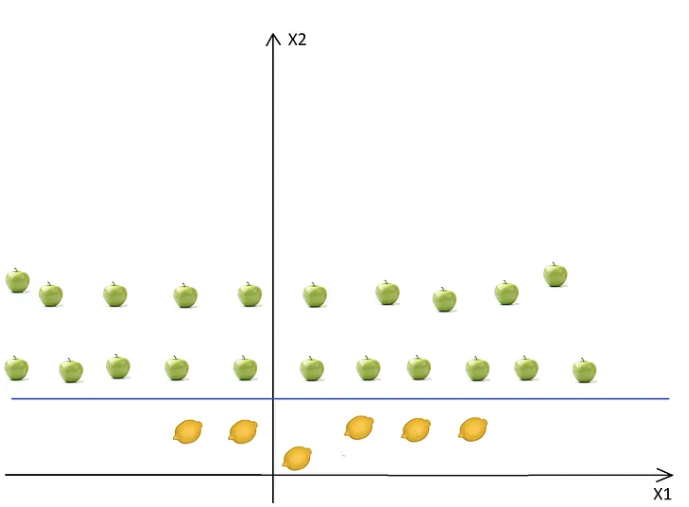
After using the kernel and after all the transformations, we will get:

Tuning parameters

Kernel

For linear kernel, the equation for prediction for a new input using the dot product between the input (x) and each support vector (xi) is calculated as follows:

f(x) = B(0) + sum(ai * (x,xi))

As a rule of thumb, always check if you have linear data, and in that case, always use linear SVM (linear kernel).
Linear SVM is a parametric model, but an RBF kernel SVM isn’t, so the complexity of the latter grows with the size of the training set.
Not only is more expensive to train an RBF kernel SVM, but you also have to keep the kernel matrix around, and the projection into this “infinite” higher dimensional space where the data becomes linearly separable is more expensive as well during prediction.
Furthermore, you have more hyperparameters to tune, so model selection is more expensive as well! And finally, it’s much easier to overfit a complex model!

Regularization

The Regularization Parameter (in Python, it’s called C) tells the SVM optimization how much you want to avoid miss classifying each training example.

If the C is higher, the optimization will choose a smaller margin hyperplane, so the training data miss classification rate will be lower.
- When the C is high, the boundary is full of curves, and all the training data was classified correctly.
On the other hand, if the C is low, then the margin will be big, even if there will be miss classified training data examples.
- As you can see in the image when the C is low, the margin is higher (so implicitly we don’t have so many curves, the line doesn’t strictly follows the data points) even if two apples were classified as lemons.
This is shown in the following two diagrams:

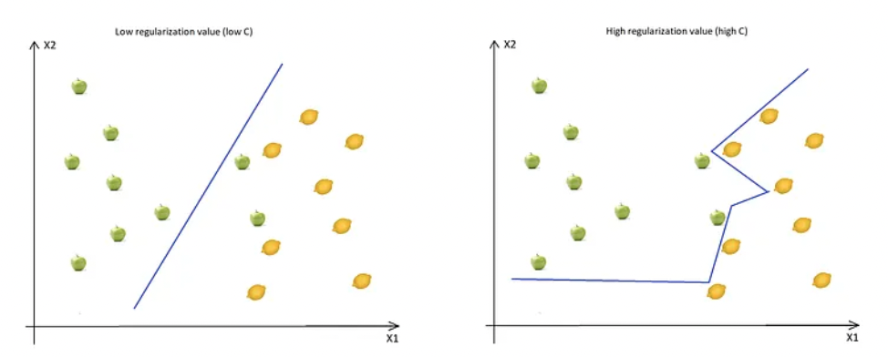
Don’t forget even if all the training data was correctly classified, this doesn’t mean that increasing the C will always increase the precision (because of overfitting).

Gamma

The gamma parameter defines how far the influence of a single training example reaches.

This means that high Gamma will consider only points close to the plausible hyperplane, and low Gamma will consider points at greater distances.

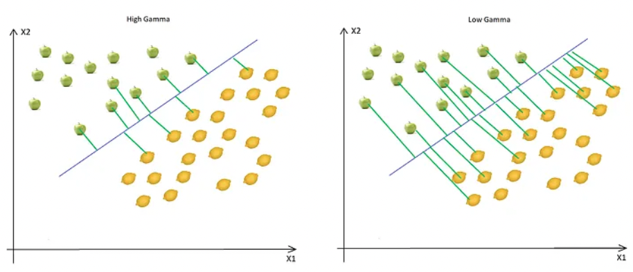
As you can see, decreasing the Gamma will result in finding the correct hyperplane will consider points at greater distances, so more and more points will be used (green lines indicate which points were considered when finding the optimal hyperplane).

Margin

Higher margin results in a better model, so better classification (or prediction). The margin should be always maximized.

SVM_Reference

K-Nearest Neighbors

Supervised machine learning algorithm as target variable is known.
Nonparametric, as it does not make an assumption about the underlying data distribution pattern
A Lazy algorithm such as KNN does not have a training step. All data points will be used only at the time of prediction. With no training step, the prediction step is costly. An eager learner algorithm eagerly learns during the training step.
Used for both Classification and Regression
Uses feature similarity to predict the cluster that the new point will fall into.

What is K in KNN?

K is a number used to identify similar neighbors for the new data point.

KNN takes K’s nearest neighbors to decide where the new data point belongs.
This decision is based on feature similarity.

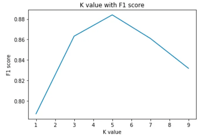
How do we choose the value of K?

The choice of K has a drastic impact on the results we obtain from KNN.

we can take the test set and plot the accuracy rate or F1 score against different values of K.

We see a high error rate for the test set when K=1. Hence we can conclude that model overfits when k=1.

For a high value of K, we see that the F1 score starts to drop. The test set reaches a minimum error rate when k=5. This is very similar to the elbow method used in K-means.

The value of K at the elbow of the test error rate gives us the optimal value of K.

We can evaluate the accuracy of the KNN classifier using K-fold cross-validation.

How does KNN work?

We have age and experience in an organization along with the salaries. We want to predict the salary of a new candidate whose age and experience are available.

Step 1: Choose a value for K. K should be an odd number.
Step 2: Find the distance of the new point to each of the training data.
Step 3:Find the K nearest neighbors to the new data point.
Step 4: For classification, count the number of data points in each category among the k neighbors. The New data point will belong to the class that has the most neighbors.

For regression, value for the new data point will be the average of the k neighbors.

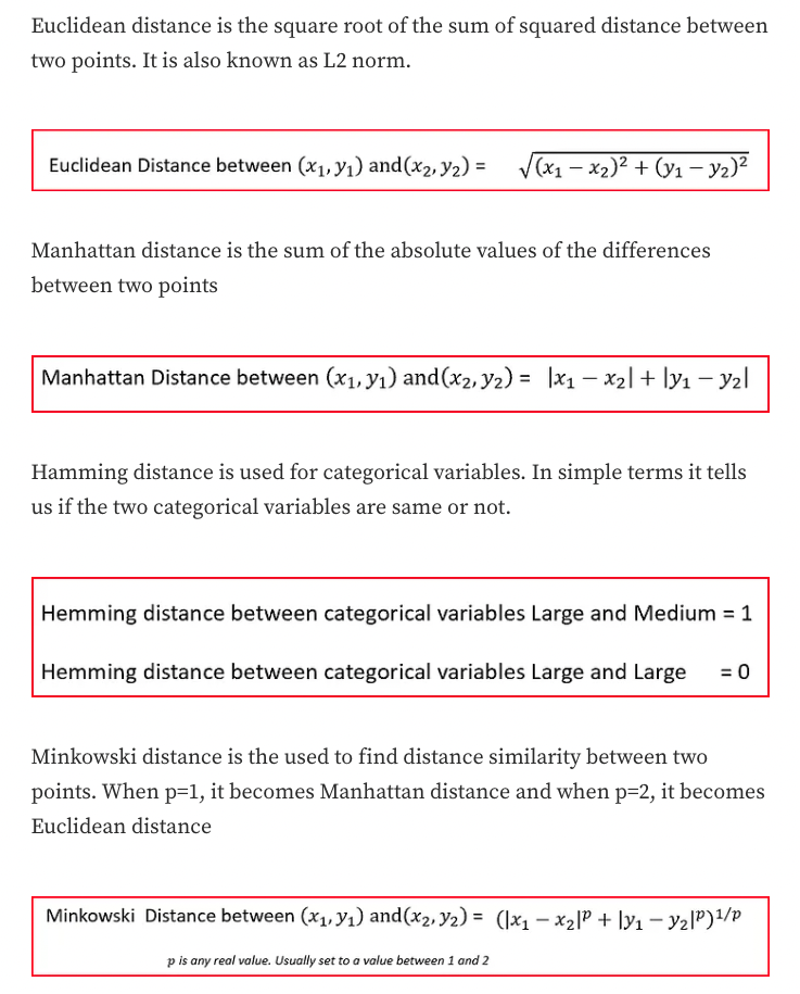
How is the distance calculated?

The distance can be calculated using many types of distances.

Pros

Simple algorithm and hence easy to interpret the prediction
Nonparametric, so it makes no assumption about the underlying data pattern
used for both classification and Regression
The training step is much faster for the nearest neighbor compared to other machine-learning algorithms

Cons

KNN is computationally expensive as it searches the nearest neighbors for the new point at the prediction stage
High memory requirement as KNN has to store all the data points
The prediction stage is very costly
Sensitive to outliers, accuracy is impacted by noise or irrelevant data.

KNN Reference

Share on

Twitter Facebook LinkedIn