PCA

Eigenvectors and Eigenvalues

How can we handle this trade-off between simplicity and the amount of information? The answer to this question is the result of the Principal Components Analysis (PCA).

Principal components can be geometrically seen as the directions of high-dimensional data, which capture the maximum amount of variance and project it onto a smaller dimensional subspace while keeping most of the information.

• The first principal component accounts for the largest possible variance; the second component will, intuitively, account for the second largest variance (under one condition: it has to be uncorrelated with the first principal component), and so forth.

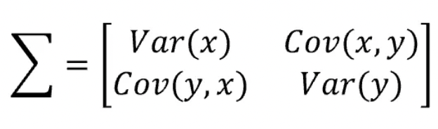
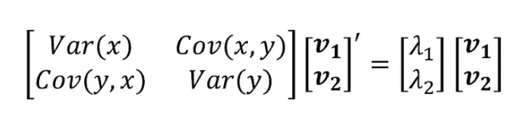
• As you can see, the covariance matrix defines both the spread (variance) and the orientation (covariance) of our data.
• The vector will point into the direction of the larger spread of data, the number will be equal to the spread (variance) of that direction.

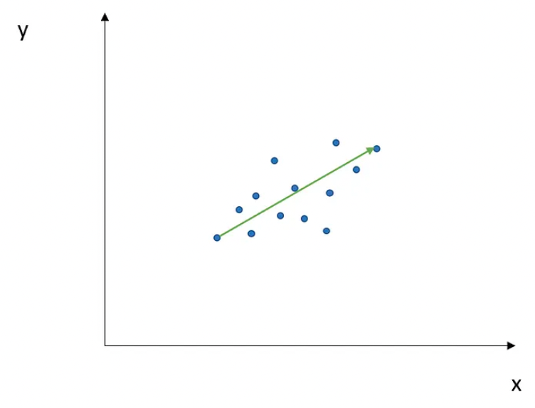
• The direction in green is the eigenvector, and it has a corresponding value, called eigenvalue, which describes its magnitude.

• Each eigenvector has a correspondent eigenvalue.
• Now, if we consider our matrix Σ and collect all the corresponding eigenvectors into a matrix V (where the number of columns, which are the eigenvectors, will be equal to the number of rows of Σ), we will obtain something like that:
• 
• 
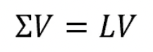
• If we sort our eigenvectors in descending order with respect to their eigenvalues, we will have that the first eigenvector accounts for the largest spread among data, the second one for the second largest spread, and so forth (under the condition that all these new directions, which describe a new space, are independent hence orthogonal among each other).

Singular vectors & singular values

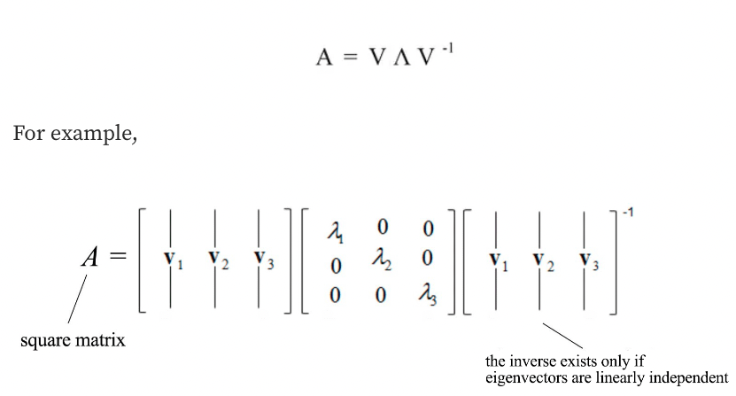
• A matrix can be diagonalized if A is a $n \times n$ a square matrix and A has n linearly independent eigenvectors.

  

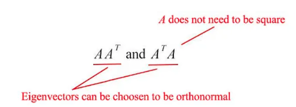
• The matrix $AA^{\top}$ and $A^{\top}A$ are very special in linear algebra.

• Consider any m × n matrix $A$. The matrices $AA^{\top}$ and $A^{\top}A$ are

  • symmetrical,

  • square,

  • at least positive semidefinite (eigenvalues are zero or positive),

  • both matrices have the same positive eigenvalues, and

  • both have the same rank $r$ as $A$.
  • 
• $u_i$: The eigenvectors for $AA^{\top}$
• $v_i$: The eigenvectors for $A^{\top}A$ as vᵢ
• Singular vectors of A: These sets of eigenvectors u and v
• Singular values: Both matrices have the same positive eigenvalues. The square roots of these eigenvalues are called Singular values.
• We concatenate vectors uᵢ into U and vᵢ into V to form orthogonal matrices.
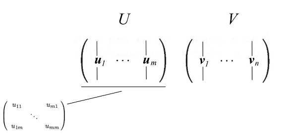
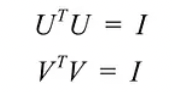
• Since these vectors are orthonormal, it is easy to prove that U and V obey

SVD

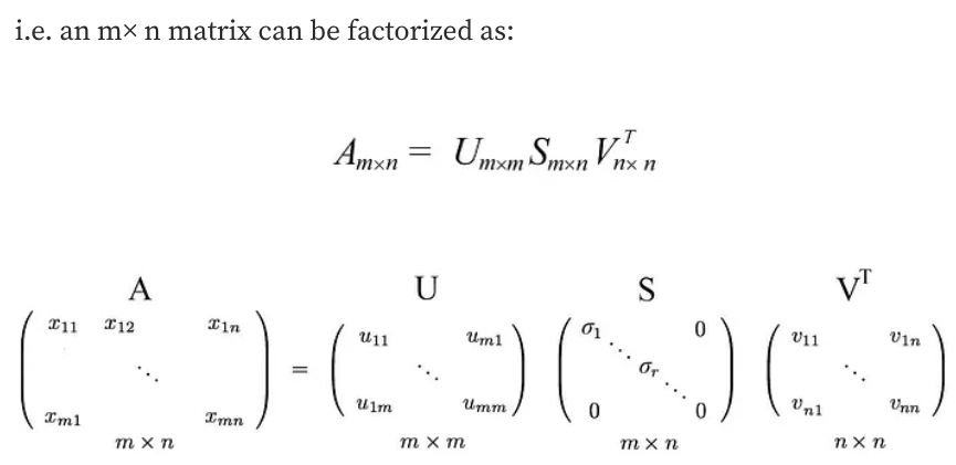
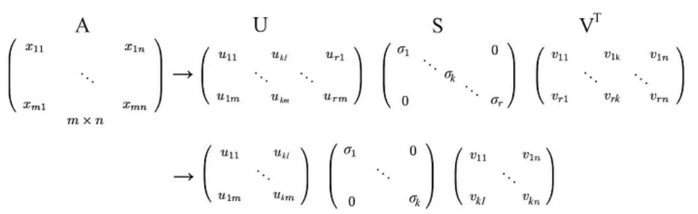
SVD states that any matrix A can be factorized as:

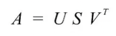
where U and V are orthogonal matrices with orthonormal eigenvectors chosen from $AA^{\top}$ and $A^{\top}A$ respectively.

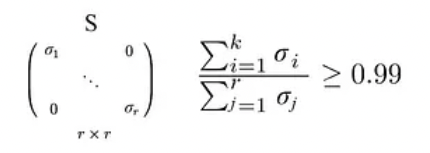
$S$ is a diagonal matrix with r elements equal to the root of the positive eigenvalues of $AA^{\top}$or $A^{\top}A$ (both matrics have the same positive eigenvalues anyway). The diagonal elements are composed of singular values.

We can arrange eigenvectors in different orders to produce U and V. To standardize the solution, we order the eigenvectors such that vectors with higher eigenvalues come before those with smaller values.

• Compared to eigendecomposition, SVD works on non-square matrices.
• U and V are invertible for any matrix in SVD, and they are orthonormal, which we love it.
• Without proof here, we also tell you that singular values are more numerically stable than eigenvalues.

Visualization

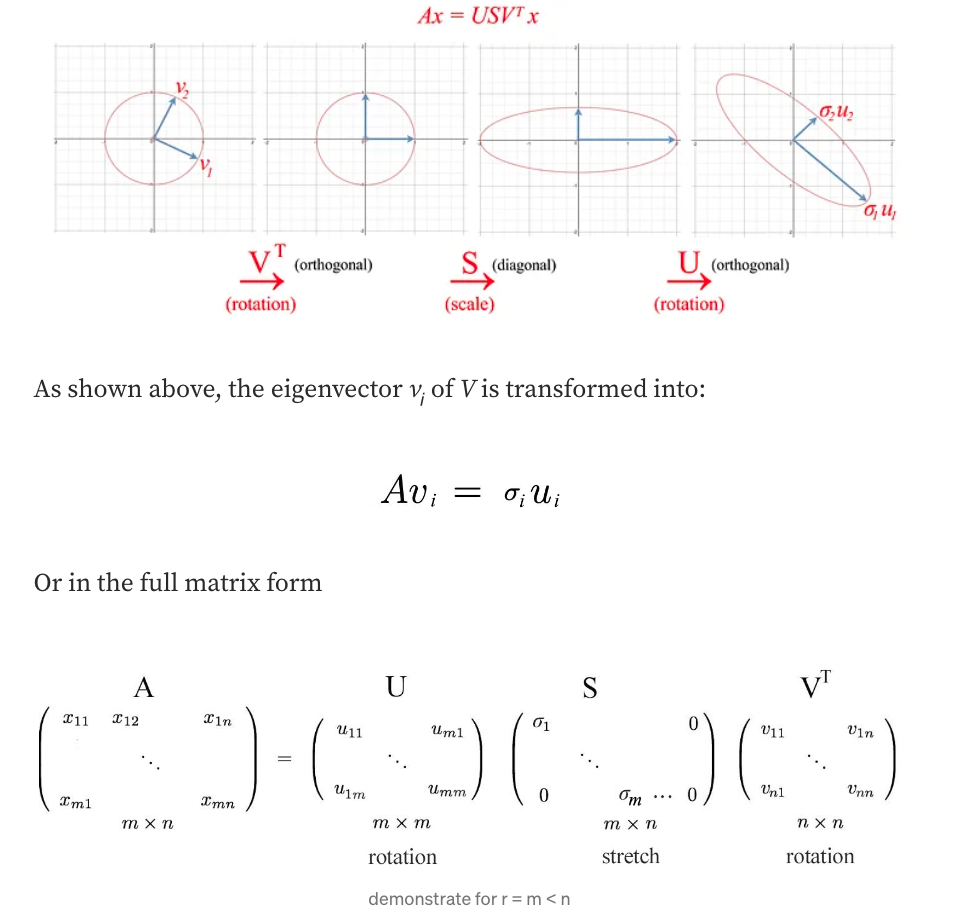
Let’s visualize what SVD does and develop the insight gradually. SVD factorizes a matrix A into USVᵀ. Applying A to a vector x (Ax) can be visualized as performing a rotation (Vᵀ), a scaling (S), and another rotation (U) on x.

Insight of SVD

The SVD can be formulated as

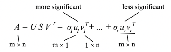
• Since uᵢ and vᵢ have unit length, the most dominant factor in determining the significance of each term is the singular value σᵢ.
• We purposely sort σᵢ in descending order. If the eigenvalues become too small, we can ignore the remaining terms (+ σᵢuᵢvᵢᵀ + …).
• 

Tips

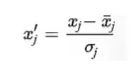
1. Scale features before performing SVD.
   1. 
2. we want to retain 99% variance, we can choose k such that
   1. 

PCA

Technically, SVD extracts data in the directions with the highest variances respectively. Obviously, we can use SVD to find PCA by truncating the less important basis vectors in the original SVD matrix.

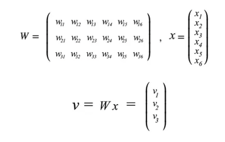
• PCA is a linear model in mapping m-dimensional input features to k-dimensional latent factors (k principal components).
• If we ignore the less significant terms, we remove the components that we care less about but keep the principal directions with the highest variances (largest information).
• 
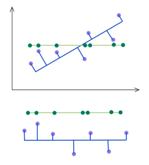
• SVD selects a projection that maximizes the variance of their output. Hence, PCA will pick the blue line over the green line if it has a higher variance.
  • 
• As indicated below, we keep the eigenvectors that have the top kth highest singular value.
  • 

Reference1