Optimization Algorithm

Gradient Descent (GD)

Gradient descent (GD) is an iterative first-order optimization algorithm used to minimize the cost function.

• The function has to be differentiable and convex.

  • Typical non-differentiable functions have a cusp or a discontinuity.

  • where 0 < lambda <1.

• Gradient Descent Algorithm iteratively calculates the next point using gradient at the current position, scales it (by a learning rate) and subtracts obtained value from the current position (makes a step).

• We implement this formula by taking the derivative (the tangential line to a function) of our cost function. The slope of the tangent line is the value of the derivative at that point and it will give us a direction to move towards. We make steps down the cost function in the direction with the steepest descent.

• 

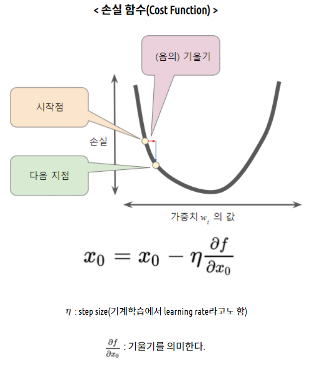
where eta controls the step size.

• The smaller learning rate the longer GD converges, or may reach maximum iteration before reaching the optimum point. On the other hand, if learning rate is too big the algorithm may not converge to the optimal point (jump around) or even to diverge completely.

This function takes 5 parameters:

1. starting point - in our case, we define it manually but in practice, it is often a random initialisation

2. gradient function - has to be specified before-hand

3. learning rate - scaling factor for step sizes

4. maximum number of iterations

5. tolerance to conditionally stop the algorithm (in this case a default value is 0.01)

Learning rate

It determines the size of the steps that are taken by the gradient descent algorithm.

If the learning rate is too big, the loss will bounce around and may not reach the local minimum.

If the learning rate is too small then gradient descent will eventually reach the local minimum but require a long time to do so.

The cost function should decrease over time if gradient descent is working properly.

Pros and cons

• A simple algorithm that is easy to implement and each iteration is cheap; we just need to compute a gradient

• However, it’s often slow because many interesting problems are not strongly convex

• Cannot handle non-differentiable functions (biggest downside)

import numpy as np

def gradient_descent(start, gradient, learn_rate, max_iter, tol=0.01):
  steps = [start] # history tracking
  x = start

  for _ in range(max_iter):
    diff = learn_rate*gradient(x)
    if np.abs(diff)<tol:
      break    
    x = x - diff
    steps.append(x) # history tracing

  return steps, x

A quadratic function

def func1(x):
  return x**2-4*x+1

def gradient_func1(x):
  return 2*x - 4

history, result = gradient_descent(9, gradient_func1, 0.1, 100)

A function with a saddle point

Disadvantage: The problem with gradient descent is that converging to a local minimum takes extensive time and determining a global minimum is not guaranteed.

The existence of a saddle point imposes a real challenge for the first-order gradient descent algorithms like GD and obtaining a global minimum is not guaranteed. Second-order algorithms deal with these situations better (e.g. Newton-Raphson method).

Stochastic Gradient Descent

In SGD, we use one training sample at each iteration instead of using the whole dataset to sum all for every step, that is — SGD performs a parameter update for each observation.

• So instead of looping over each observation, it just needs one to perform the parameter update.

• In SGD, before for-looping, we need to randomly shuffle the training examples.

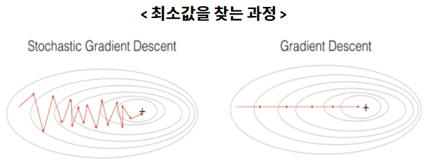
• SGD is usually faster than batch gradient descent, but its path to the minima is more random than batch gradient descent since SGD uses only one example at a time.

• SGD is widely used for larger dataset training, computationally faster, and can allow for parallel model training because it has to have a memory for one sample.

Mini-Batch Gradient Descent

• Splitting the training data into smaller batches.

• Rather than calculating the gradient of a single training example, the gradient is calculated against a batch size of n training examples (Mini-batch gradient descent uses n data points (instead of one sample in SGD) at each iteration.).

• Samples in each gradient calculation: consecutive subsets of the dataset

Batch size

• mini Batch: equally sized subsets of the dataset over which the gradient is calculated and weights updated (A subset of all your data during one iteration).

Epoch

• One loop over the entire training dataset.

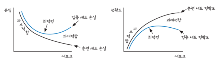
• Too many epochs can lead to overfitting of the training dataset, whereas too few may result in an underfit model, but decrease the loss.

• Early stopping is a method that allows you to specify an arbitrarily large number of training epochs and stop training once the model performance stops improving on the validation dataset.

import numpy as np
import matplotlib.pyplot as plt
%matplotlib inline

np.random.seed(0)

X = 2 * np.random.rand(100,1)
y = 6 +4 * X+ np.random.randn(100,1)

plt.scatter(X, y)

<matplotlib.collections.PathCollection at 0x7fc1c881f0a0>

def stochastic_gradient_descent_steps(X, y, batch_size=10, iters=1000):
    w0 = np.zeros((1,1))
    w1 = np.zeros((1,1))
    prev_cost = 100000
    iter_index =0
    
    for ind in range(iters):
        np.random.seed(ind)
        #sample_X, sample_y
        stochastic_random_index = np.random.permutation(X.shape[0])
        sample_X = X[stochastic_random_index[0:batch_size]]
        sample_y = y[stochastic_random_index[0:batch_size]]
        #w1_update, w0_update
        w1_update, w0_update = get_weight_updates(w1, w0, sample_X, sample_y, learning_rate=0.01)
        w1 = w1 - w1_update
        w0 = w0 - w0_update
    
    return w1, w0

def get_weight_updates(w1, w0, X, y, learning_rate=0.01):
    N = len(y)

    w1_update = np.zeros_like(w1)
    w0_update = np.zeros_like(w0)

    y_pred = np.dot(X, w1.T) + w0
    diff = y-y_pred
         
    w0_factors = np.ones((N,1))

    w1_update = -(2/N)*learning_rate*(np.dot(X.T, diff))
    w0_update = -(2/N)*learning_rate*(np.dot(w0_factors.T, diff))    
    
    return w1_update, w0_update

def gradient_descent_steps(X, y, iters=10000):

    w0 = np.zeros((1,1))
    w1 = np.zeros((1,1))
    
    for ind in range(iters):
        w1_update, w0_update = get_weight_updates(w1, w0, X, y, learning_rate=0.01)
        w1 = w1 - w1_update
        w0 = w0 - w0_update
              
    return w1, w0

def get_cost(y, y_pred):
    N = len(y) 
    cost = np.sum(np.square(y - y_pred))/N
    return cost

w1, w0 = stochastic_gradient_descent_steps(X, y, iters=1000)
print("w1:",round(w1[0,0],3),"w0:",round(w0[0,0],3))
y_pred = w1[0,0] * X + w0
print('Stochastic Gradient Descent Total Cost:{0:.4f}'.format(get_cost(y, y_pred)))

w1: 4.028 w0: 6.156
Stochastic Gradient Descent Total Cost:0.9937

Newton-Raphson

It can be easily generalized to the problem of finding solutions of a system of non-linear equations, which is referred to as Newton’s technique.

• It requires only one inital value $x_0$, which we will refer to as the initial guess for the root.

• To see how the N-R method works, we can rewrite the function f(x) using a Taylor series expansion in (x-x0):

$f(x) = f(x_0) + f’(x_0)(x-x_0) + 1/2 f’‘(x_0)(x-x_0)^2 + … = 0 $

where f’(x) denotes the first derivative of f(x) with respect to x, f’‘(x) is the second derivative, and so forth.

• Now, suppose the initial guess is pretty close to the real root. Then (x-x0) is small, and only the first few terms in the series are important to get an accurate estimate of the true root, given x0.

• By truncating the series at the second term (linear in x), we obtain the N-R iteration formula for getting a better estimate of the true root:

• Thus the N-R method finds the tangent to the function f(x) at $x=x_0$ and extrapolates it to intersect the x axis to get $x_1$. This point of intersection is taken as the new approximation to the root and the procedure is repeated until convergence is obtained whenever possible. Mathematically, given the value of $x = x_i$ at the end of the ith iteration, we obtain $x_{i+1}$ as

Pros and cons

Pros:

• It is best method to solve the non-linear equations.

• The order of convergence is quadric i.e. of second order which makes this method fast as compared to other methods.

• It is very easy to implement on computer.

Cons:

• This method becomes complicated if the derivative of the function f(x) is not simple.

• This method requires a great and sensitive attention regarding the choice of its approximation.

def func(x):
    return x * x * x - x * x + 2
 
# Derivative of the above function
# which is 3*x^x - 2*x
def derivFunc(x):
    return 3 * x * x - 2 * x
 
# Function to find the root
def newtonRaphson(x):
    h = func(x) / derivFunc(x)
    while abs(h) >= 0.0001:
        h = func(x)/derivFunc(x)
         
        # x(i+1) = x(i) - f(x) / f'(x)
        x = x - h
     
    print("The value of the root is : ",
                             "%.4f"% x)
 
# Driver program to test above
x0 = -20 # Initial values assumed
newtonRaphson(x0)
 

The value of the root is :  -1.0000