Handling Missing Values
A perfect data set is usually a big win for any data scientist or machine learning engineer. Unfortunately, more often than not, datasets will have missing data.

Causes of Missing Data
- Data is not being intentionally filled, especially if it is an optional field.
- Data being corrupted.
- Human error.
- If it was a survey, participants might quit the survey halfway.
- If data is being automatically by computer applications, then a malfunction could cause missing data. Eg. a sensor recording logs malfunctioning.
- Fraudulent behavior of intentionally deleting data.
Types of Missing Data
- Missing Completely at Random (MCAR)
- This effectively implies that the causes of the missing data are unrelated to the data.
- It is safe to ignore many of the complexities that arise because of the missing data, apart from the obvious loss of information.
- Example: Estimate the gross annual income of a household within a certain population, which you obtain via questionnaires. In the case of MCAR, the missingness is completely random, as if some questionnaires were lost by mistake.
- Missing at Random (MAR)
- If the probability of being missing is the same only within groups defined by the observed data, then the data are missing at random (MAR).
- For instance, suppose you also collected data on the profession of each subject in the questionnaire and deduce that managers, VIPs, etc are more likely not the share their income. Then, within subgroups of the profession, missingness is random.
- Not Missing at Random (NMAR)
- If neither MCAR nor MAR holds, then we speak of missing not at random (MNAR).
- Example: In the case of MNAR when the reason for missingness depends on the missing values themselves. For instance, suppose people don’t want to share their income as it is less, and they are ashamed of it.
Ways to Handle Missing Values
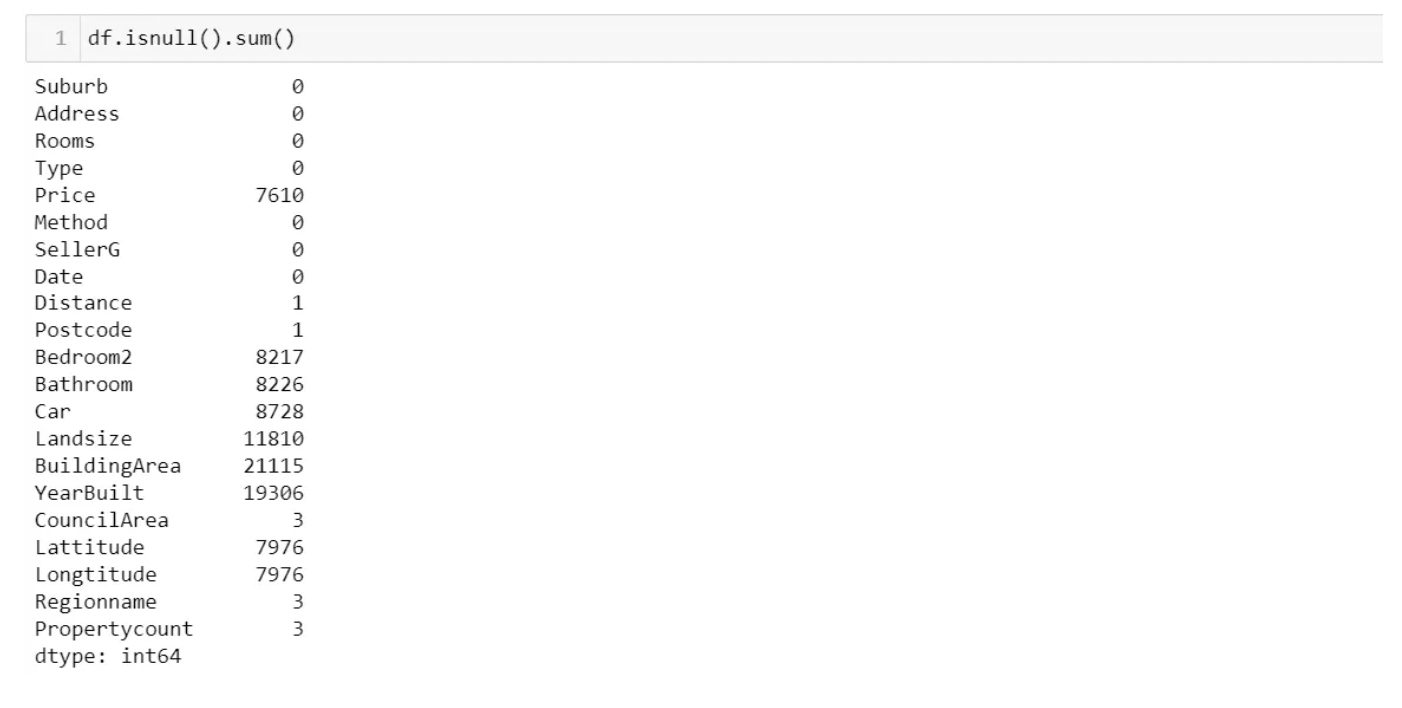
Pandas write the value NaN(Not a Number) when it finds a missing value.
Checking Missing Values
The easy way:
- Deleting rows that have missing values.
- This technique can lead to loss of information and hence should not be used when the count of rows with missing values is high.

- Deleting columns with missing values.
- If we have columns that have extremely high missing values in them (say 80% of the data in the columns is missing), then we can delete these columns.
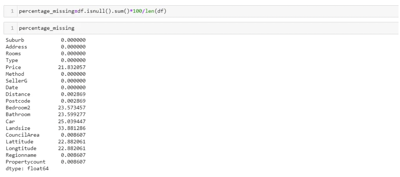
- With the above output, you can now decide to set a threshold for the percentage of the missing values you want to delete.
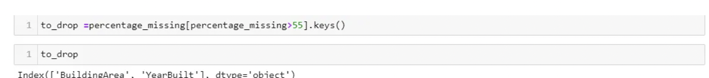
- From the output Building Area and YearBuilt are the columns we will delete using the drop function.
- It is an option only if the number of missing values is 2% of the whole dataset or less.
- Do not use this as your first approach.
- Leave it to the algorithm
- Some algorithms can factor in the missing values and learn the best imputation values for the missing data based on the training loss reduction (ie. XGBoost).
- Some others have the option to just ignore them (ie. LightGBM — use_missing=false).
- However, other algorithms throw an error about the missing values (ie. Scikit learn — LinearRegression).
- Is an option only if the missing values are about 5% or less. Works with MCAR.

The professional way:
The drawback of dropping missing values is that you loose the entire row just for the a few missing values. That is a lot of valuable data.
- Try filling in the missing values with a well-calculated estimate.
- Professionals use two main methods of calculating missing values. They are imputation and interpolation.
Imputation
Mean/Median Imputation
Numerical Data: Replacing missing values with mean, mode, or median
- Note that this method can add variance and bias error.
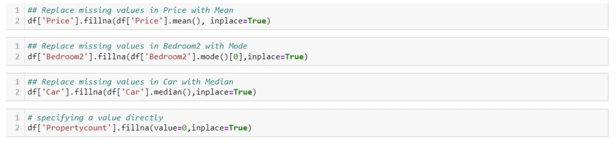
- Your business rules could also have specified values to fill your missing values with. You can just specify the value directly as well, for instance, I am replacing BuildingSize with size 100 by default for all missing values.

Advantages:
- Quick and easy
- Ideal for small numerical datasets
Disadvantages:
- Doesn’t factor in the correlations between features. It only works on the column level.
- It will give poor results on encoded categorical features (do NOT use it on categorical features).
- Not very accurate.
- Doesn’t account for the uncertainty in the imputations.
Most Frequent (Values) Imputation
Categorical Data: Replacing missing values with the most frequent
-
Imputing using mean, mode, and median works best with numerical values. For categorical data, we can impute using the most frequent or constant value.
-
Let’s use the sklearn impute package to replace categorical data with the most frequent value by specifying strategy=’most_frequent’
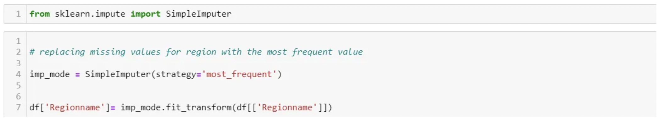 The code above will replace Regionname with the most frequent region.
 -
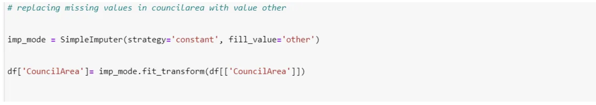
Let’s use the sklearn impute package to replace categorical data with a constant value by specifying strategy=’constant’. You also need to include which value is going to be filler by specifying the fill_value. In our case, we are going to fill missing values in column ‘CouncilArea’ with a value called ‘other’. This technique can also be used when there are set business rules for the use case in context.
-
You can now see below we have a new category called other added to the ‘CouncilArea’ column.

Advantages:
- Works well with categorical features.
Disadvantages:
- It also doesn’t factor in the correlations between features.
- It can introduce bias in the data.
Zeros Imputation
-
It replaces the missing values with either zero or any constant value you specify.
-
Perfect for when the null value does not add value to your analysis but requires an integer in order to produce results.
Regression Imputation
Instead of just taking the mean, you’re taking the predicted value based on other variables. This preserves relationships among variables involved in the imputation model but not variability around predicted values.
- Predicting missing values using algorithms
- If you want to replace a categorical value, use the classification algorithm.
- If predicting a continuous number, we use a regression algorithm. This method is also good because it generates unbiased estimates.
Stochastic Regression Imputation
The predicted value from a regression plus a random residual value. This has all the advantages of regression imputation but adds in the advantages of the random component.
Imputaiton using k-NN
- The k nearest neighbors is an algorithm that is used for simple classification.
- The algorithm uses ‘feature similarity’ to predict the values of any new data points.
- This can be very useful in making predictions about the missing values by finding the k’s closest neighbors to the observation with missing data and then imputing them based on the non-missing values in the neighborhood.
- The process is as follows: Basic mean impute -> KDTree -> compute nearest neighbors (NN) -> Weighted average.
Pros:
- Can be much more accurate than the mean, median or most frequent imputation methods (It depends on the dataset).
Cons:
- Computationally expensive. KNN works by storing the whole training dataset in memory.
- K-NN is quite sensitive to outliers in the data.
Imputation Using Multivariate Imputation by Chained Equation (MICE)
This type of imputation works by filling in the missing data multiple times. Multiple Imputations (MIs) are much better than a single imputation as it measures the uncertainty of the missing values in a better way.
The chained equations approach is also very flexible and can handle different variables of different data types (i.e., continuous or binary) as well as complexities such as bounds or survey skip patterns.
install.package("mice") #install mice
install.package("lattice")#install lattice
library("mice") #load mice
library("lattice") #load lattice

micedata <- mice(mtcars[, !names(mtcars) %in% "cyl"], method="rf")  # perform mice imputation, based on random forests.
miceOutput <- complete(micedata)  # generate the completed data.

#Check for NAs
anyNA(miceOutput)
When to use Imputation or Interpolation:
Imputation: When you require the mean or median of a set of values.
Eg, If there are missing values in a dataset of marks obtained by students, you can impute missing values with the mean of the other student’s marks.
Interpolation: When you have data points with a linear relationship.
Eg: The growth chart of a healthy child. The child will grow taller with each passing year until they are 16. Any missing values along this growth chart will be part of a straight line, so the missing values can be interpolated.
Leave a comment