Feature Selection

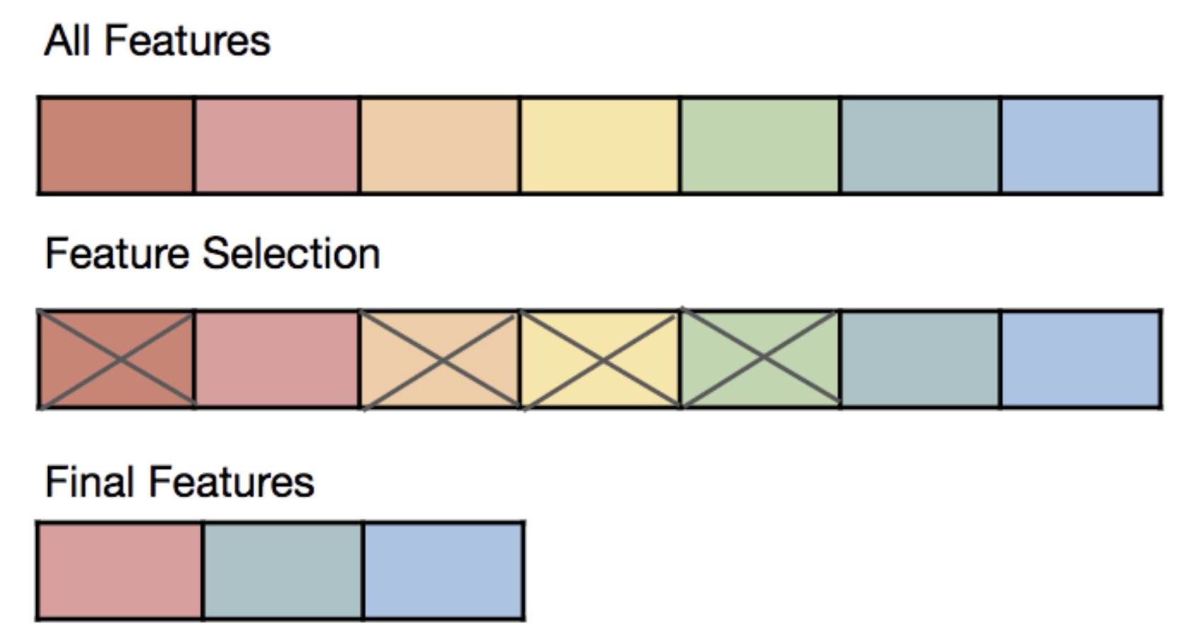
Selecting which features to use is a crucial step in any machine learning project and a recurrent task in the day-to-day of a Data Scientist.

• Two of the biggest problems in Machine Learning are
  • Overfitting (fitting aspects of data that are not generalizable outside the dataset)
  • the Curse of dimensionality (the unintuitive and sparse properties of data in high dimensions).
• Feature selection helps to avoid both of these problems by reducing the number of features in the model and trying to optimize the model performance.
• In doing so, feature selection also provides an extra benefit: Model interpretation. With fewer features, the output model becomes simpler and easier to interpret, and it becomes more likely for a human to trust future predictions made by the model.

Unsupervised methods

• One simple method to reduce the number of features consists of applying a Dimensionality Reduction technique to the data.
• Dimensionality reduction does not actually select a subset of features but instead produces a new set of features in a lower dimension space.
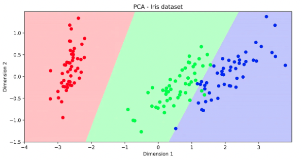
• In practice, we perform dimensionality reduction (e.g. PCA) over a subset of features and check how the labels are distributed in the reduced space. If they appear to be separate, this is a clear sign that high classification performance is expected when using this set of features.

from sklearn.datasets import load_iris
from sklearn.decomposition import PCA
from sklearn.svm import SVC
import matplotlib.pyplot as plt
from matplotlib.colors import ListedColormap
import numpy as np
h = .01
x_min, x_max = -4,4
y_min, y_max = -1.5,1.5
# loading dataset
data = load_iris()
X, y = data.data, data.target
# selecting first 2 components of PCA
X_pca = PCA().fit_transform(X)
X_selected = X_pca[:,:2]
# training classifier and evaluating on the whole plane
clf = SVC(kernel='linear')
clf.fit(X_selected,y)
xx, yy = np.meshgrid(np.arange(x_min, x_max, h),
                     np.arange(y_min, y_max, h))
Z = clf.predict(np.c_[xx.ravel(), yy.ravel()])
Z = Z.reshape(xx.shape)
# Plotting
cmap_light = ListedColormap(['#FFAAAA', '#AAFFAA', '#AAAAFF'])
cmap_bold = ListedColormap(['#FF0000', '#00FF00', '#0000FF'])
plt.figure(figsize=(10,5))
plt.pcolormesh(xx, yy, Z, alpha=.6,cmap=cmap_light)
plt.title('PCA - Iris dataset')
plt.xlabel('Dimension 1')
plt.ylabel('Dimension 2')
plt.scatter(X_pca[:,0],X_pca[:,1],c=data.target,cmap=cmap_bold)
plt.show()

Univariate filter methods

• Filter methods aim at ranking the importance of the features without making use of any type of classification algorithm.
• Univariate filter methods evaluate each feature individually and do not consider feature interactions.
• The scores usually either measure the dependency between the dependent variable and the features (e.g. Chi2 and, for regression, Pearls correlation coefficient), or the difference between the distributions of the features given the class label (F-test and T-test).
• Understanding these assumptions is important to decide which test to use, even though some of them are robust to violations of the assumptions.
• Scores based on statistical tests provide a p-value, that may be used to rule out some features. This is done if the p-value is above a certain threshold (typically 0.01 or 0.05).

from sklearn.feature_selection import f_classif, chi2, mutual_info_classif
from statsmodels.stats.multicomp import pairwise_tukeyhsd
from sklearn.datasets import load_iris
data = load_iris()
X,y = data.data, data.target
chi2_score, chi_2_p_value = chi2(X,y)
f_score, f_p_value = f_classif(X,y)
mut_info_score = mutual_info_classif(X,y)
pairwise_tukeyhsd = [list(pairwise_tukeyhsd(X[:,i],y).reject) for i in range(4)]
print('chi2 score        ', chi2_score)
print('chi2 p-value      ', chi_2_p_value)
print('F - score score   ', f_score)
print('F - score p-value ', f_p_value)
print('mutual info       ', mut_info_score)
print('pairwise_tukeyhsd',pairwise_tukeyhsd)
Out:
chi2 score         [ 10.82   3.71 116.31  67.05]
chi2 p-value       [0.   0.16 0.   0.  ]
F - score score    [ 119.26   49.16 1180.16  960.01]
F - score p-value  [0. 0. 0. 0.]
mutual info        [0.51 0.27 0.98 0.98]
pairwise_tukeyhsd [[True, True, True], [True, True, True], [True, True, True], [True, True, True]]

Visual ways to rank features

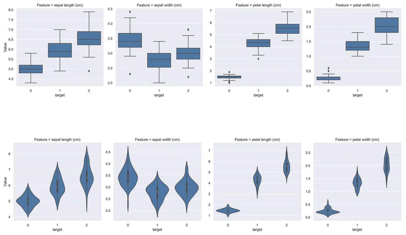
Boxplots and Violin plots

• Boxplots / Violin plots may help to visualize the distribution of the feature given the class. For the Iris dataset, an example is shown below.

• This is useful in that statistical tests often only evaluate the difference between the mean of such distributions. These plots, therefore, provide more information about the quality of the features

import pandas as pd
import seaborn as sns
sns.set()
df = pd.DataFrame(data.data,columns=data.feature_names)
df['target'] = data.target
df_temp = pd.melt(df,id_vars='target',value_vars=list(df.columns)[:-1], 
                  var_name="Feature", value_name="Value")
g = sns.FacetGrid(data = df_temp, col="Feature", col_wrap=4, size=4.5,sharey = False)
g.map(sns.boxplot,"target", "Value");
g = sns.FacetGrid(data = df_temp, col="Feature", col_wrap=4, size=4.5,sharey = False)
g.map(sns.violinplot,"target", "Value");

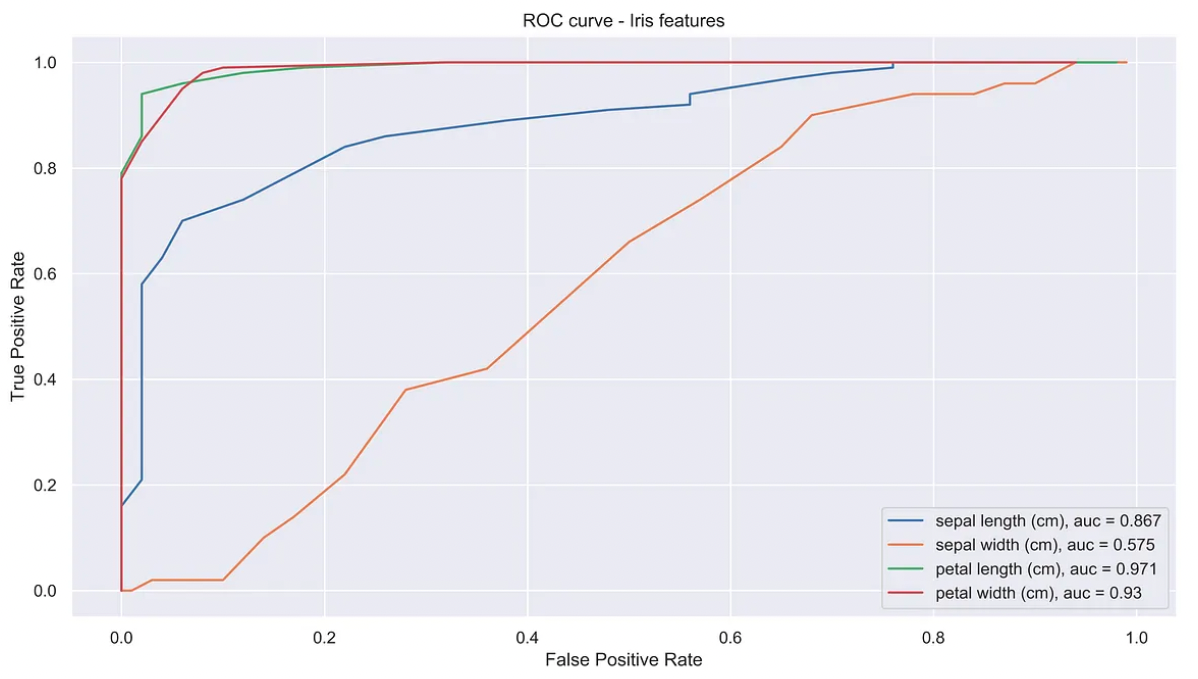
Feature Ranking with the ROC curve

• The ROC curve may be used to rank features in importance order, which gives a visual way to rank features performances.

• This technique is most suitable for binary classification tasks. To apply in problems with multiple classes this, one could use micro or macro averages or multiple comparison based criteria (similarly to the pairwise Tukey’s range test).

• The example below plots the ROC curve of various features.

from sklearn.datasets import load_iris
import matplotlib.pyplot as plt
from sklearn.metrics import auc
import numpy as np
# loading dataset
data = load_iris()
X, y = data.data, data.target
y_ = y == 2
plt.figure(figsize=(13,7))
for col in range(X.shape[1]):
    tpr,fpr = [],[]
    for threshold in np.linspace(min(X[:,col]),max(X[:,col]),100):
        detP = X[:,col] < threshold
        tpr.append(sum(detP & y_)/sum(y_))# TP/P, aka recall
        fpr.append(sum(detP & (~y_))/sum((~y_)))# FP/N
        
    if auc(fpr,tpr) < .5:
        aux = tpr
        tpr = fpr
        fpr = aux
    plt.plot(fpr,tpr,label=data.feature_names[col] + ', auc = '\
                           + str(np.round(auc(fpr,tpr),decimals=3)))
plt.title('ROC curve - Iris features')
plt.xlabel('False Positive Rate')
plt.ylabel('True Positive Rate')
plt.legend()
plt.show()

Multivariate Filter methods

• These methods take into account the correlations between variables and do so without considering any type of classification algorithm.

mRMR

mRMR (minimum Redundancy Maximum Relevance) is a heuristic algorithm to find a close to optimal subset of features by considering both the features importances and the correlations between them.

• Even if two features are highly relevant, it may not be a good idea to add both of them to the feature set if they are highly correlated.
• In that case, adding both features would increase the model complexity (increasing the possibility of overfitting) but would not add significant information, due to the correlation between the features.
• In a set S of N features, the relevance of the features (D) is computed as follows:
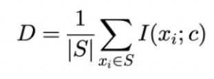  • where I is the mutual information operator.
• The redundancy of the features is denoted as follows:
• The mRMR score for the set S is defined as (D - R).
• The goal is to find the subset of features with a maximum value of (D-R).
• In practice, however, we perform an incremental search (aka forward selection) in which, at each step, we add the feature that yields the greatest mRMR.
• A (not maintained) python wrapper was created on the name pymrmr. In case of issues with pymrmr, I advise calling the C — level function directly.

import pandas as pd
import pymrmr
df = pd.read_csv('some_df.csv')
# Pass a dataframe with a predetermined configuration. 
# Check http://home.penglab.com/proj/mRMR/ for the dataset requirements
pymrmr.mRMR(df, 'MIQ', 10)

*** This program and the respective minimum Redundancy Maximum Relevance (mRMR)
     algorithm were developed by Hanchuan Peng <hanchuan.peng@gmail.com>for
     the paper
     "Feature selection based on mutual information: criteria of
      max-dependency, max-relevance, and min-redundancy,"
      Hanchuan Peng, Fuhui Long, and Chris Ding,
      IEEE Transactions on Pattern Analysis and Machine Intelligence,
      Vol. 27, No. 8, pp.1226-1238, 2005.
*** MaxRel features ***
 Order    Fea     Name    Score
 1        765     v765    0.375
 2        1423    v1423   0.337
 3        513     v513    0.321
 4        249     v249    0.309
 5        267     v267    0.304
 6        245     v245    0.304
 7        1582    v1582   0.280
 8        897     v897    0.269
 9        1771    v1771   0.269
 10       1772    v1772   0.269
*** mRMR features ***
 Order    Fea     Name    Score
 1        765     v765    0.375
 2        1123    v1123   24.913
 3        1772    v1772   3.984
 4        286     v286    2.280
 5        467     v467    1.979
 6        377     v377    1.768
 7        513     v513    1.803
 8        1325    v1325   1.634
 9        1972    v1972   1.741
 10       1412    v1412   1.689
Out[1]:
 ['v765',
  'v1123',
  'v1772',
  'v286',
  'v467',
  'v377',
  'v513',
  'v1325',
  'v1972',
  'v1412']

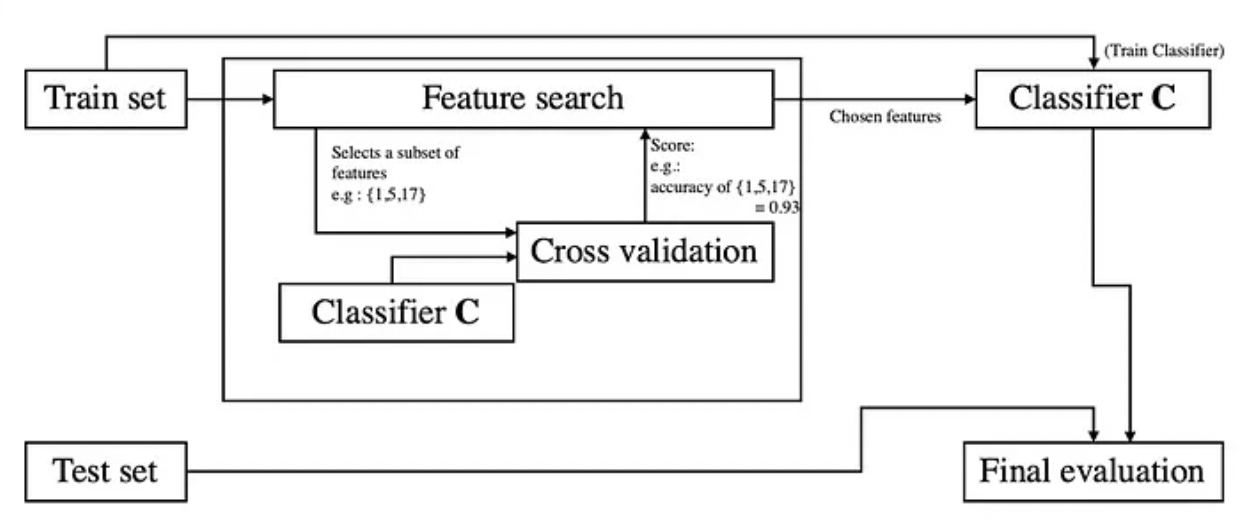
Wrapper methods

The main idea behind a wrapper method is to search which set of features works best for a specific classifier.

1. Choose a performance metric (Likelihood, AIC, BIC, F1-score, accuracy, MSE, MAE…), noted as M.
2. Choose a classifier / regressor / … , noted as C in here.
3. Search different features subsets with a given search method. For each subset S, do the following:

• Train and test C in a cross-validation pattern, using S as the classifier’s features;
• Obtain the average score from the cross-validation procedure (for the metric M) and assign this score to the subset S;
• Choose a new subset and redo step a.

Detailing Step 3

Step three leaves unspecified the type which search method will be used. Testing all possible subsets of features is prohibitive (Brute Force selection) in virtually any situation since it would require performing step 3 an exponential number of times (2 to the power of the number of features). Besides the time complexity, with such a large number of possibilities, it would be likely that a certain combination of features performs best simply by random chance, which makes the brute force solution more prone to overfitting.

Search Algorithm

• Search algorithms tend to work well in practice to solve this issue.

• They tend to achieve a performance close to the brute force solution, with much less time complexity and less chance of overfitting.

• Forward selection and Backward selection (aka pruning) are much used in practice.

  • Backward selection consists of starting with a model with the full number of features and, at each step, removing the feature without which the model has the highest score.
  • Forward selection goes on the opposite way: it starts with an empty set of features and adds the feature that best improves the current score.

• Forward/Backward selection are still prone to overfitting, as, usually, scores tend to improve by adding more features.

  • One way to avoid such situation is to use scores that penalize the complexity of the model, such as AIC or BIC.

  

Step three also leaves open the cross-validation parameters. Usually, a k-fold procedure is used. Using a large k, however, introduces extra complexity to the overall wrapper method.

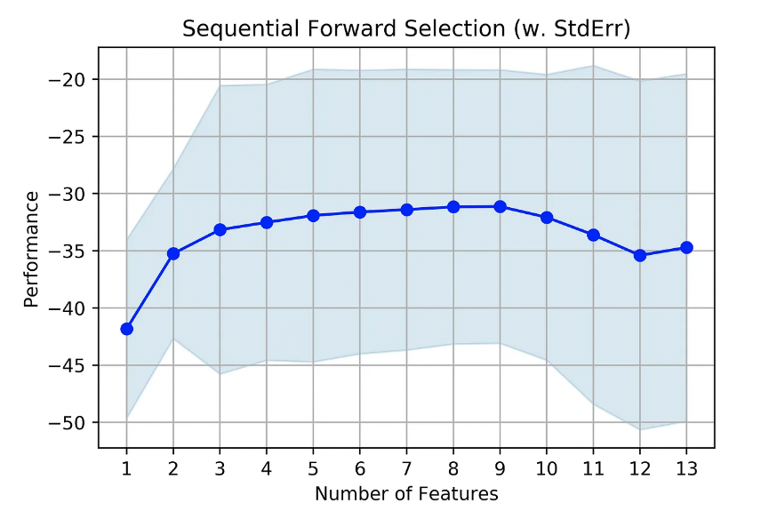
A Python Package for wrapper methods

mlxtend (http://rasbt.github.io/mlxtend/) is a useful package for diverse data science-related tasks. The wrapper methods on this package can be found on SequentialFeatureSelector. It provides Forward and Backward feature selection with some variations.

The package also provides a way to visualize the score as a function of the number of features through the function plot_sequential_feature_selection.

The example below was extracted from the package’s main page.

from mlxtend.feature_selection import SequentialFeatureSelector as SFS
from mlxtend.plotting import plot_sequential_feature_selection as plot_sfsfrom sklearn.linear_model import LinearRegression
from sklearn.datasets import load_bostonboston = load_boston()
X, y = boston.data, boston.targetlr = LinearRegression()sfs = SFS(lr, 
          k_features=13, 
          forward=True, 
          floating=False, 
          scoring='neg_mean_squared_error',
          cv=10)sfs = sfs.fit(X, y)
fig = plot_sfs(sfs.get_metric_dict(), kind='std_err')plt.title('Sequential Forward Selection (w. StdErr)')
plt.grid()
plt.show()

Embedded methods

Training a classifier boils down to an optimization problem, where we try to minimize a function of its parameters (noted here as 𝜃). This function is known loss function (noted as 𝐿(𝜃)).

In a more general framework, we usually want to minimize an objective function that takes into account both the loss function and a penalty (or regularisation)(Ω(𝜃)) to the complexity of the model:

obj(𝜃)=𝐿(𝜃)+Ω(𝜃)

Embedded methods for Linear classifiers

For linear classifiers (e.g. Linear SVM, Logistic Regression), the loss function is noted as :

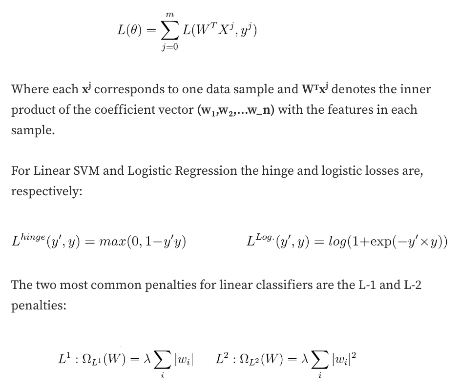
• The higher the value of λ, the stronger the penalty and the optimal objective function will tend to end up in shrinking more and more the coefficients w_i.
• The “L1” penalty is known to create sparse models, which simply means that, it tends to select some features out of the model by making some of the coefficients equal zero during the optimization process.
• While L-2 shrinks the coefficients and therefore helps avoid overfitting, it does not create sparse models, so it is not suitable as a feature selection technique.
• For some linear classifiers (Linear SVM, Logistic Regression), the L-1 penalty can be efficiently used, meaning that there are efficient numerical methods to optimize the resulting objective function. The same is not true for several other classifiers (various Kernel SVM methods, Decision Trees,…). Therefore, different regularization methods should be used for different classifiers.

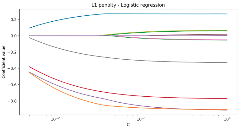
An example of Logistic regression with regularisation is shown below, and we can see that the algorithms rule out some of the features as C decreases (think if C as 1/λ).

import numpy as np
import matplotlib.pyplot as plt
from sklearn.svm import LinearSVC
from sklearn.model_selection import ShuffleSplit
from sklearn.model_selection import GridSearchCV
from sklearn.utils import check_random_state
from sklearn import datasets
from sklearn.linear_model import LogisticRegression
rnd = check_random_state(1)
# set up dataset
n_samples = 3000
n_features = 15
# l1 data (only 5 informative features)
X, y = datasets.make_classification(n_samples=n_samples,
                                        n_features=n_features, n_informative=5,
                                        random_state=1)
cs = np.logspace(-2.3, 0, 50)
coefs = []
for c in cs:
    clf = LogisticRegression(solver='liblinear',C=c,penalty='l1')
    # clf = LinearSVC(C=c,penalty='l1', loss='squared_hinge', dual=False, tol=1e-3)
    
    clf.fit(X,y)
    coefs.append(list(clf.coef_[0]))
    
coefs = np.array(coefs)
plt.figure(figsize=(10,5))
for i,col in enumerate(range(n_features)):
    plt.plot(cs,coefs[:,col])
plt.xscale('log')
plt.title('L1 penalty - Logistic regression')
plt.xlabel('C')
plt.ylabel('Coefficient value')
plt.show()

Feature importances from tree-based models

Another common feature selection technique consists in extracting a feature importance rank from tree base models.

The feature importances are essentially the mean of the individual trees’ improvement in the splitting criterion produced by each variable. In other words, it is how much the score (so-called “impurity” on the decision tree notation) was improved when splitting the tree using that specific variable.

They can be used to rank features and then select a subset of them. However, the feature importances should be used with care, as they suffer from biases and, and presents an unexpected behavior regarding highly correlated features regardless of how strong they are.

As shown in this paper, random forest feature importances are biased towards features with more categories. Besides, if two features are highly correlated, both of their scores largely decrease, regardless of the quality of the features.

Below is an example of how to extract the feature importances from a random forest. Although a regressor, the process would be the same for a classifier.

from sklearn.datasets import load_boston
from sklearn.ensemble import RandomForestRegressor
import numpy as np
boston = load_boston()
X = boston.data
Y = boston.target
feat_names = boston.feature_names 
rf = RandomForestRegressor()
rf.fit(X, Y)
print("Features sorted by their score:")
print(sorted(zip(map(lambda x: round(x, 4), rf.feature_importances_), feat_names), 
             reverse=True))
Out:
Features sorted by their score:
[(0.4334, 'LSTAT'), (0.3709, 'RM'), (0.0805, 'DIS'), (0.0314, 'CRIM'), (0.0225, 'NOX'), (0.0154, 'TAX'), (0.0133, 'PTRATIO'), (0.0115, 'AGE'), (0.011, 'B'), (0.0043, 'INDUS'), (0.0032, 'RAD'), (0.0016, 'CHAS'), (0.0009, 'ZN')]

Extra: main Impurity scores for tree models

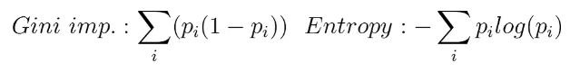
As explained above, the “impurity” is a score used by the decision tree algorithm when deciding to split a node. There are many decision tree algorithms (IDR3, C4.5, CART,…), but the general rule is that the variable with which we split a node in the tree is the one that generates the highest improvement on the impurity.

The most common impurities are the Gini Impurity and Entropy. An improvement on the Gini impurity is known as “Gini importance” while An improvement on the Entropy is the Information Gain.

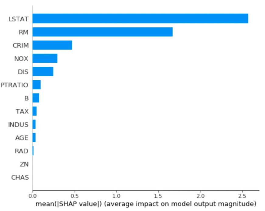
SHAP: Reliable feature importances from tree models

SHAP is actually much more than just that. It is an algorithm to provide model explanation out of any predictive model. For tree based models, however, it is specially useful: the authors developed a high speed and exact (not only local) explanation for such models, compatible with XGBoost, LightGBM, CatBoost, and scikit-learn tree models.

I encourage checking out the explanation capabilities provided by SHAP (such as Feature dependance, interaction effects, model monitoring…). Below, I plot (only) the feature importances output by SHAP, which are more reliable than those output by the original tree model when ranking them for feature selection. This example was extracted from their github page.

import xgboost
import shap# load JS visualization code to notebook
shap.initjs()# train XGBoost model
X,y = shap.datasets.boston()
model = xgboost.train({"learning_rate": 0.01}, xgboost.DMatrix(X, label=y), 100)# explain the model's predictions using SHAP values
# (same syntax works for LightGBM, CatBoost, and scikit-learn models)
explainer = shap.TreeExplainer(model)
shap_values = explainer.shap_values(X)shap.summary_plot(shap_values, X, plot_type="bar")

Conclusion

Embedded methods are usually very efficient to avoid overfitting and select useful variables. They are also time efficient as they are embedded on the objective function. Their main downside is that they may not be available to the desired classifier.

Wrapper methods tend to work very well in practice. However, they are computationally expensive, specially when dealing hundreds of features. But if you have the computational resources, they are an excellent way to go.

If the feature set is very large (on the order of hundreds or thousands), because filter methods are fast, they can work well as a first stage of selection, to rule out some variables. Subsequently another method can be applied to the already reduced feature set. This is particular useful if you want to create combinations of features, multiplying or dividing them, for example.

Reference1