Evaluation

We summarize how well a supervised model performs on a given dataset.

Accuracy

Classification accuracy is a metric that summarizes the performance of a classification model as the number of correct predictions / the total number of predictions.

• But, Accuracy is not a good metric of predictive performance for imbalanced data.

Imbalanced data refers to a problem where the distribution of examples across classes is biased.

The machine learning algorithms favor the larger class and sometimes even ignore the smaller class if the data is highly imbalanced.

import pandas as pd
import numpy as np
import matplotlib.pyplot as plt
import mglearn

from sklearn.datasets import load_digits
from sklearn.model_selection import train_test_split
from sklearn.linear_model import LogisticRegression

import warnings
warnings.filterwarnings('ignore')

from sklearn.metrics import accuracy_score

digits = load_digits()
y = digits.target == 9
X_train, X_test, y_train, y_test = train_test_split(digits.data, y, random_state=0)

logreg = LogisticRegression(C=0.1).fit(X_train, y_train)
pred_logreg = logreg.predict(X_test)
print("logreg score: {:.2f}".format(logreg.score(X_test, y_test)))
print("Accuracy score: {:.2f}".format(accuracy_score(y_test, pred_logreg)))

logreg score: 0.98
Accuracy score: 0.98

Imbalanced example

Let’s suppose that we have two classes: C0 and C1.

• X ~ N(0, 4), Y~N(2, 1)
• Suppose also that class C0 represents 90% of the dataset (and, so, class C1 represents the remaining 10%).
• In the following picture, we have depicted a representative dataset containing 50 points along with the theoretical distributions of both classes in the right proportions.

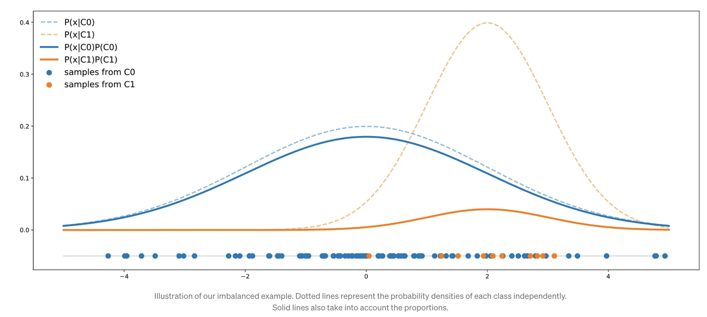
• The curve of the C0 class is always above the curve of the C1 class.
• Using Bayes rule,
• From a perfect theoretical point of view, if we had to train a classifier on these data, the accuracy of the classifier would be maximal when always answering C0.

However, we can notice that facing an imbalanced dataset doesn’t necessarily mean that the two classes are not well separable (they are not far apart from each other).

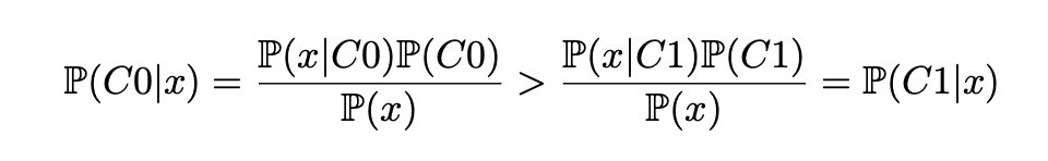
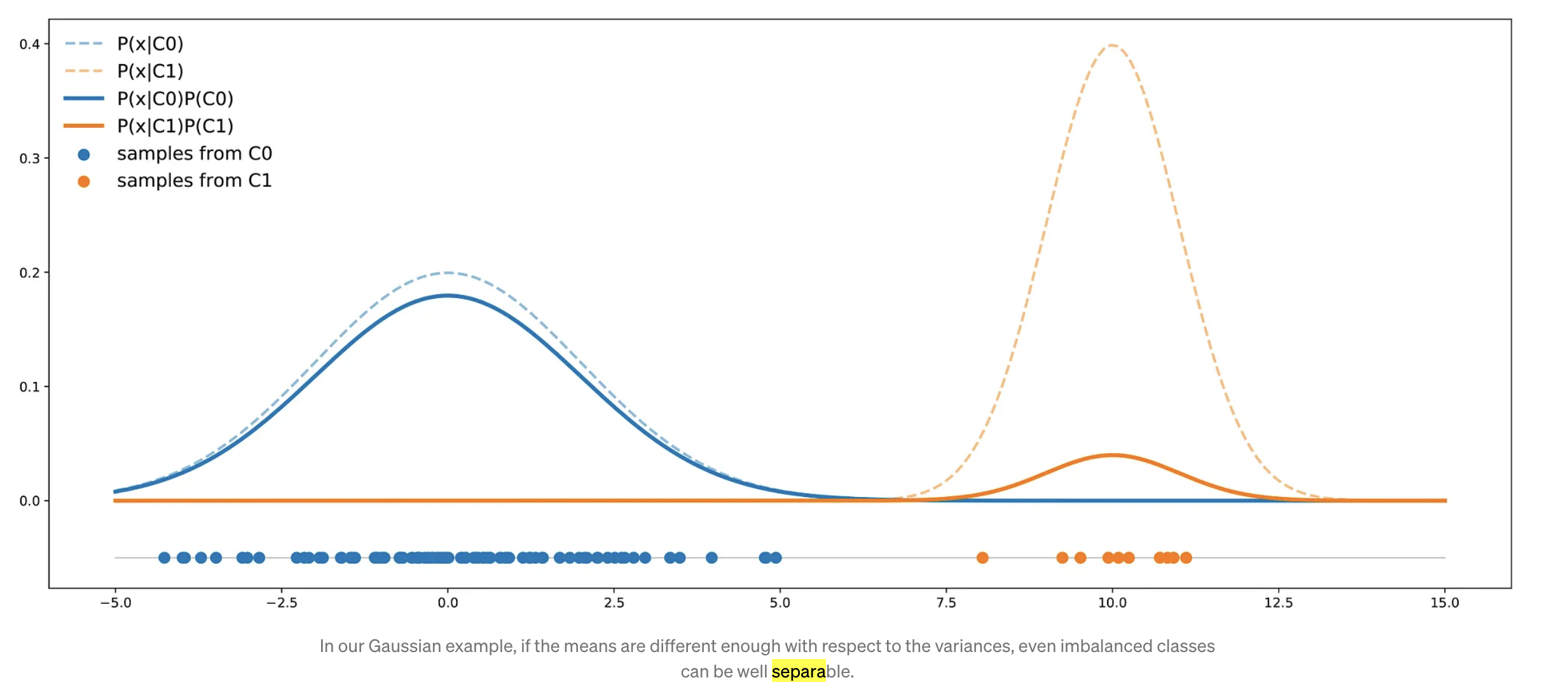
• Consider that we still have two classes C0 (90%) and C1 (10%).
• X ~ N(0, 4), Y~N(10, 1)

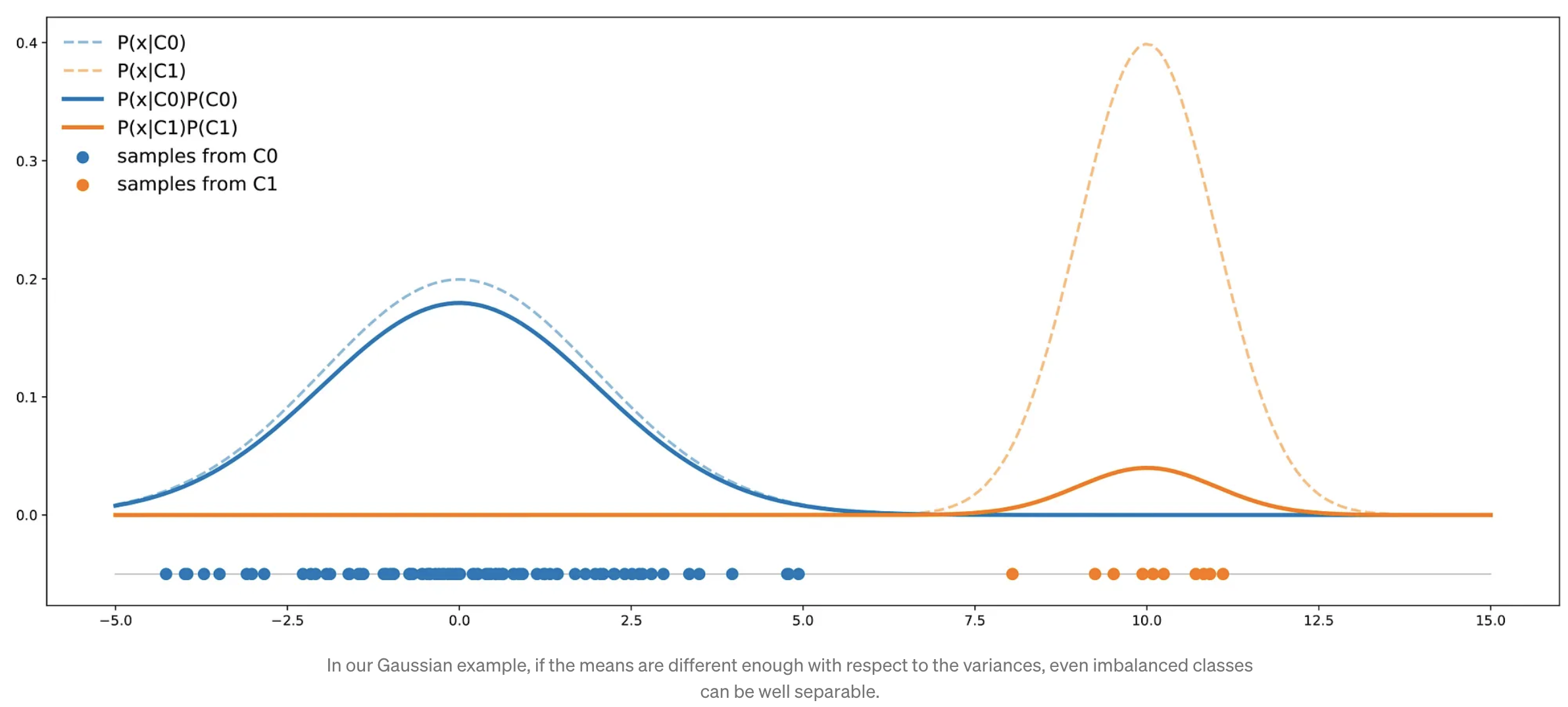
• In this case, the two classes are separated enough to compensate for the imbalance: a classifier will not necessarily answer C0 all the time.
• When dealing with an imbalanced dataset, if classes are not well separable with the given variables and if our goal is to get the best possible accuracy, the best classifier can be a “naive” one that always answers the majority class.

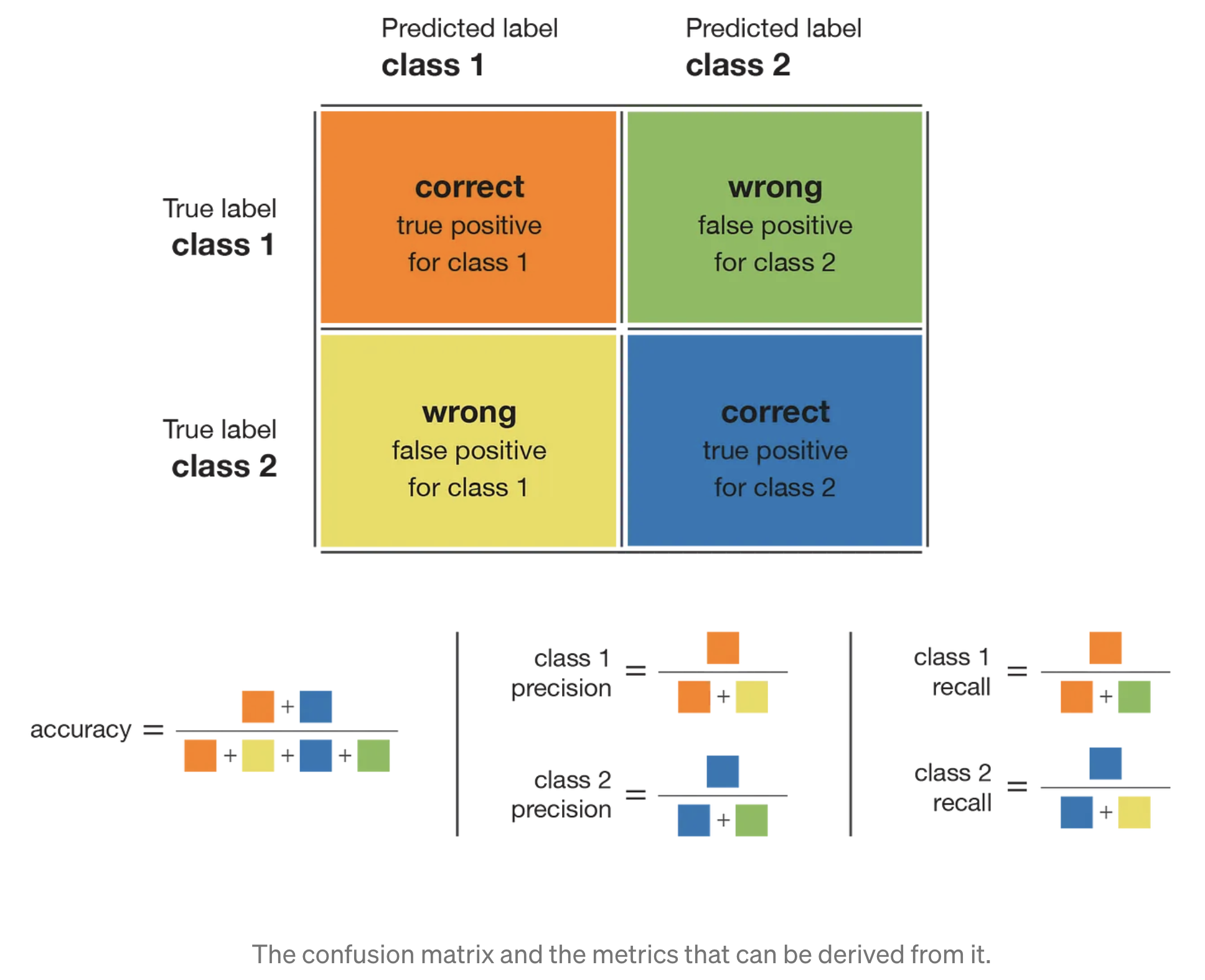
Confusion matrices

mglearn.plots.plot_binary_confusion_matrix()

The test is negative, the patient will be assumed healthy, while if the test is positive, the patient will undergo additional screening. We can’t assume that our model will always work perfectly, and it will make mistakes.

• False positive (type I error): An incorrect positive prediction

A type I error occurs if an investigator rejects a null hypothesis that is actually true in the population.

• False negative (type II error): An incorrect negative prediction

A type II error occurs if the investigator fails to reject a null hypothesis that is actually false in the population.

Types of errors play an important role when one of two classes is much more frequent than the other one.

Now let’s say you build a classifier that is 99% accurate on the click prediction task. What does that tell you? 99% accuracy sounds impressive, but this doesn’t consider the class imbalance. You can achieve 99% accuracy without building a machine-learning model by always predicting “no click.” On the other hand, even with imbalanced data, a 99% accurate model could be quite good. However, accuracy doesn’t allow us to distinguish the constant “no click” model from a potentially good model.

from sklearn.metrics import confusion_matrix

confusion = confusion_matrix(y_test, pred_logreg)
print("Confusion matrix:\n{}".format(confusion))

Confusion matrix:
[[402   1]
 [  6  41]]

• It has more true positives and true negatives while having fewer false positives and false negatives.

• From this comparison, it is clear that only the decision tree and the logistic regression give reasonable results, and that the logistic regression works better than the tree on all accounts.

• However, inspecting the full confusion matrix is a bit cumbersome, and while we gained a lot of insight from looking at all aspects of the matrix, the process was very manual and qualitative.

• There are several ways to summarize

the information in the confusion matrix: Accuracy, Precision, recall, and f-score.

Precision

Precision measures how many of the samples predicted as positive are actually positive:

\[Precision = \frac{TP}{TP + FP}.\]

• Precision is used as a performance metric when the goal is to limit the number of false positives.
• The precision of a class defines how trustable the result is when the model answers that a point belongs to that class.

For example, imagine a model for predicting whether a new drug will effectively treat a disease in clinical trials.

Clinical trials are notoriously expensive, and a pharmaceutical company will only want to run an experiment if it is very sure that the drug will actually work.

Therefore, it is important that the model does not produce many false positives—in other words, that it has a high precision.

from sklearn.metrics import precision_score

print("Precision score: {:.2f}".format(precision_score(y_test, pred_logreg)))

Precision score: 0.98

Recall (Sensitivity)

Recall, on the other hand, measures how many of the positive samples are captured by the positive predictions:

\[Recall = \frac{TP}{TP + FN}.\]

• Recall is used as performance metric when we need to identify all positive samples; that is, when it is important to avoid false negatives.
• The recall of a class expresses how well the model is able to detect that class.

The cancer diagnosis example is a good example of this: it is important to find all people that are sick, possibly including healthy patients in the prediction.

from sklearn.metrics import recall_score

print("Recall score: {:.2f}".format(recall_score(y_test, pred_logreg)))

Recall score: 0.87

• high recall + high precision : the class is perfectly handled by the model
• low recall + high precision : the model can’t detect the class well but is highly trustable when it does
• high recall + low precision : the class is well detected but the model also include points of other classes in it
• low recall + low precision : the class is poorly handled by the model

Trade-off between recall and precision

There is a trade-off between optimizing recall and optimizing precision.

• You can trivially obtain a perfect recall if you predict all samples to belong to the positive class— there will be no false negatives and no true negatives either.

• However, predicting all samples as positive will result in many false positives, and therefore the precision will be very low.

• If you find a model that predicts only the single data point it is most sure about as positive and the rest as negative, then precision will be perfect (assuming this data point is positive), but recall will be terrible.

F1-score

while precision and recall are very important measures, looking at only one of them will not provide you with the full picture. One way to summarize them is the f1-score, which is the harmonic mean of precision and recall:

\[F_1 = \frac{2}{\frac{1}{recall} + \frac{1}{precision}} = 2 \cdot \frac{precision\cdot recall}{precision + recall}.\]

from sklearn.metrics import f1_score

print("f1 score logistic regression: {:.2f}".format(
f1_score(y_test, pred_logreg)))

f1 score logistic regression: 0.92

• The f1-score seems to capture our intuition of what makes a good model much better than accuracy did.

• Disadvantage: it is harder to interpret and explain than accuracy.

from sklearn.metrics import classification_report
print(classification_report(y_test, pred_logreg,
target_names=["not nine", "nine"]))

              precision    recall  f1-score   support

    not nine       0.99      1.00      0.99       403
        nine       0.98      0.87      0.92        47
    
    accuracy                           0.98       450
   macro avg       0.98      0.93      0.96       450
weighted avg       0.98      0.98      0.98       450

Precision-recall curve

Changing the threshold that is used to make a classification decision in a model is a way to adjust the trade-off of precision and recall for a given classifier.

• Setting a requirement on a classifier like 90% recall is often called setting the operating point.

• Often, when developing a new model, it is not entirely clear what the operating point will be.

• For this reason, and to understand a modeling problem better, it is informative to look at all possible thresholds or all possible trade-offs of precision and recalls at once: Precision-recall curve

from sklearn.metrics import precision_recall_curve

precision, recall, thresholds = precision_recall_curve(
y_test, pred_logreg)

close_zero = np.argmin(np.abs(thresholds-9))
plt.plot(precision[close_zero], recall[close_zero], 'o', markersize=10,
label="threshold zero", fillstyle="none", c='k', mew=2)
plt.plot(precision, recall, label="precision recall curve")
plt.xlabel("Precision")
plt.ylabel("Recall")
plt.legend(loc="best")

<matplotlib.legend.Legend at 0x7fb800589df0>

ROC curve

Similar to the precision-recall curve, the ROC curve considers all possible thresholds for a given classifier, but instead of reporting precision and recall, it shows the false positive rate (FPR) against the true positive rate (TPR).

\[TPR = recall = \frac{TP}{TP + FN}.\]

The false positive rate is the fraction of false positives out of all negative samples.

\[FPR = \frac{FP}{FP + TN}.\]

sklearn.plots.plot_binary_confusion_matrix()

from sklearn.metrics import roc_curve

fpr, tpr, thresholds = roc_curve(y_test, pred_logreg)
plt.plot(fpr, tpr, label="ROC Curve")
plt.plot([0, 1], [0, 1], 'k--', label = 'Random')
plt.xlabel("FPR")
plt.ylabel("TPR (recall)")

plt.legend(loc=4)

<matplotlib.legend.Legend at 0x7fb7e0373e50>

For the ROC curve, the ideal curve is close to the top left: you want a classifier that produces a high recall while keeping a low false positive rate.

• A good AUROC score means that the model we are evaluating does not sacrifice a lot of precision to get a good recall of the observed class (often the minority class).

• Compared to the default threshold of 0, the curve shows that we can achieve a significantly higher recall (around 0.9) while only increasing the FPR slightly.

• Be aware that choosing a threshold should not be done on the test set but on a separate validation set.

• Because AUC is the area under a curve that goes from 0 to 1, AUC always returns a value between 0 (worst) and 1 (best).

• Predicting randomly always produces an AUC of 0.5, no matter how imbalanced the classes in a dataset are. This makes AUC a much better metric for imbalanced classification problems than accuracy.

The AUC can be interpreted as evaluating the ranking of positive samples.

It’s equivalent to the probability that a randomly picked point of the positive class will have a higher score according to the classifier than a randomly picked point from the negative class.

So, a perfect AUC of 1 means that all positive points have a higher score than all negative points. For classification problems with imbalanced classes, using AUC for model selection is often much more meaningful than using accuracy.

from sklearn.svm import SVC
from sklearn.metrics import roc_auc_score

y = digits.target == 9
X_train, X_test, y_train, y_test = train_test_split(
digits.data, y, random_state=0)
plt.figure()
for gamma in [1, 0.05, 0.01]:
    svc = SVC(gamma=gamma).fit(X_train, y_train)
    accuracy = svc.score(X_test, y_test)
    auc = roc_auc_score(y_test, svc.decision_function(X_test))
    fpr, tpr, _ = roc_curve(y_test , svc.decision_function(X_test))
    print("gamma = {:.2f} accuracy = {:.2f} AUC = {:.2f}".format(
        gamma, accuracy, auc))
    plt.plot(fpr, tpr, label="gamma={:.3f}".format(gamma))
plt.xlabel("FPR")
plt.ylabel("TPR")
plt.xlim(-0.01, 1)
plt.ylim(0, 1.02)
plt.legend(loc="best")

gamma = 1.00 accuracy = 0.90 AUC = 0.50
gamma = 0.05 accuracy = 0.90 AUC = 1.00
gamma = 0.01 accuracy = 0.90 AUC = 1.00

<matplotlib.legend.Legend at 0x7fb800538ee0>

A perfect AUC of 1 means that all positive points have a higher score than all negative points.

Undersampling, oversampling and generating synthetic data

• Undersampling consists in sampling from the majority class in order to keep only a part of these points
• Oversampling consists in replicating some points from the minority class in order to increase its cardinality
• Generating synthetic data consists in creating new synthetic points from the minority class (see SMOTE method for example) to increase its cardinality