Data Preprocessing

Encoding for Categorical variables

• Most Machine learning algorithms can not handle categorical variables unless we convert them to numerical values.
• Feature engineering is essential, yet it is also arguably one of the most manually intensive steps in the applied ML process.
• Handling non-numeric data is a critical component of nearly every machine-learning process.
• Many algorithms’ performances vary based on how Categorical variables are encoded.
• Categorical variables can be divided into two categories: Nominal (No particular order: Red, Yellow, Pink, Blue) and Ordinal (some ordered: Red, Yellow, Pink, Blue).
• My recommendation will be to try each of these with the smaller datasets and then decide where to focus on tuning the encoding process.

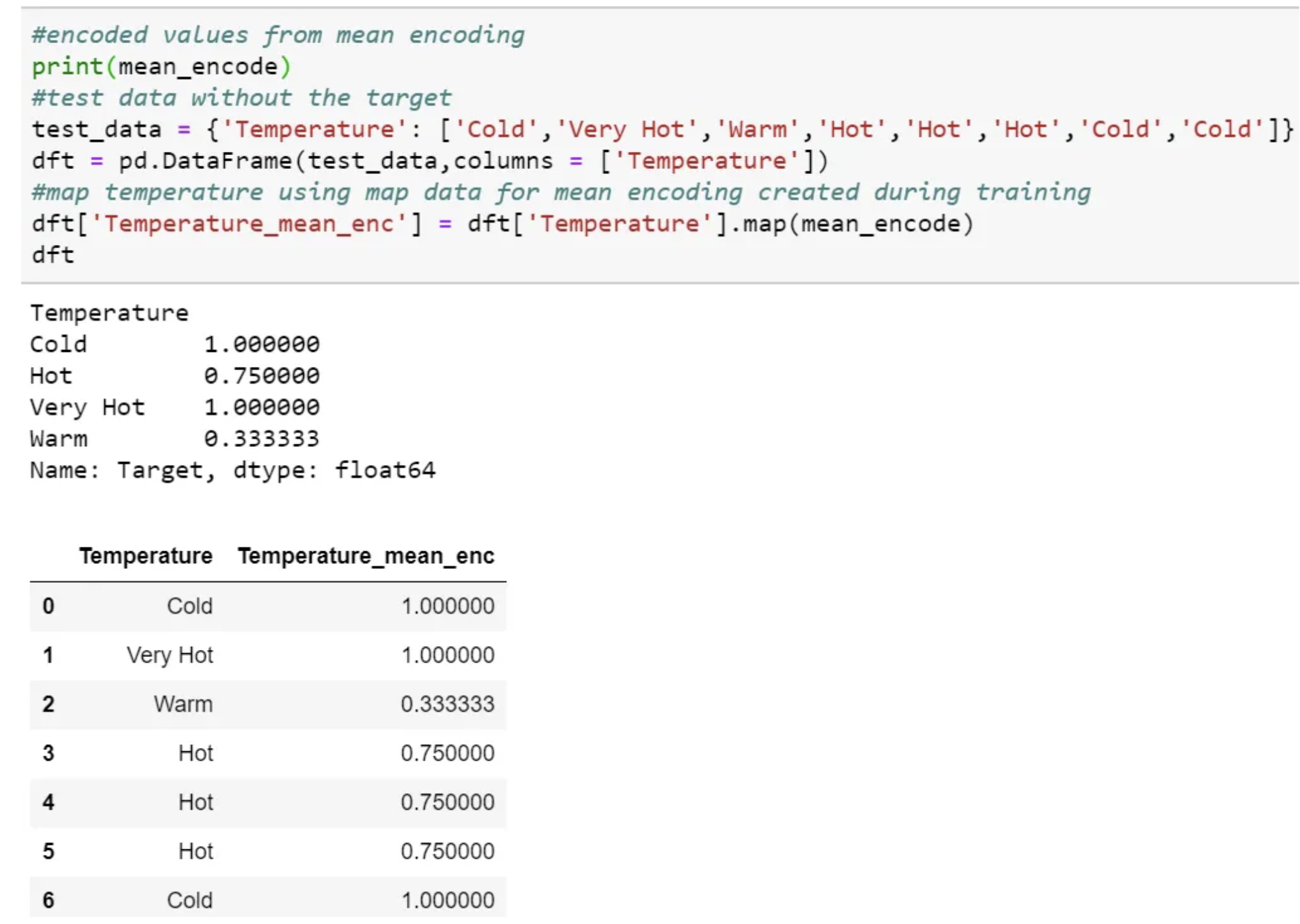
We need to use the mapping values created at the time of training.

This process is the same as scaling or normalization, where we use the train data to scale or normalize the test data.

Then map and use the same value in testing time pre-processing.

We can even create a dictionary for each category and map the value and then use the dictionary at testing time.

One Hot encoding

By far, the most common way to represent categorical variables is using the one-hot encoding or one-out-of-N encoding, also known as dummy variables.

• We map each category to a vector that contains 1 and 0, denoting the presence or absence of the feature.
• The number of vectors depends on the number of categories for features.
• Cons: This method produces many columns that slow down the learning significantly if the number of the category is very high for the feature.

from sklearn.preprocessing import LabelEncoder
from sklearn.preprocessing import OneHotEncoder
import numpy as np
import pandas as pd
items = ['TV', 'Fridge', 'Microwave', 'Computer', 'Fan', 'Fan', 'Blender', 'Blender']

le = LabelEncoder()
le.fit(items)
labels = le.transform(items).reshape(-1, 1)

print(le.transform(items))

ohe = OneHotEncoder()
ohe.fit(labels)
ohe_labels = ohe.transform(labels)
print(ohe_labels.toarray())
print(ohe_labels.shape)

[5 3 4 1 2 2 0 0]
[[0. 0. 0. 0. 0. 1.]
 [0. 0. 0. 1. 0. 0.]
 [0. 0. 0. 0. 1. 0.]
 [0. 1. 0. 0. 0. 0.]
 [0. 0. 1. 0. 0. 0.]
 [0. 0. 1. 0. 0. 0.]
 [1. 0. 0. 0. 0. 0.]
 [1. 0. 0. 0. 0. 0.]]
(8, 6)

• When working with data that was input by humans (say, users on a website), there might not be a fixed set of categories, and differences in spelling and capitalization might require preprocessing.

• Check the contents of a column.

pd.DataFrame(items).value_counts()

Blender      2
Fan          2
Computer     1
Fridge       1
Microwave    1
TV           1
dtype: int64

We can represent all categories by N-1 (N= No of Category) as sufficient to encode the one that is not included.

• Usually, for Regression, we use N-1 (drop the first or last column of One Hot Coded new feature ).
  • The linear Regression has access to all of the features as it is being trained and therefore examines the whole set of dummy variables altogether.
  • This means that N-1 binary variables give complete information about (represent completely) the original categorical variable to the linear Regression.
• Still, for classification, the recommendation is to use all N columns, as most of the tree-based algorithm builds a tree based on all available variables.

The get_dummies function

The get_dummies function automatically transforms all columns that have object type (like strings) or are categorical.

• Pandas has get_dummies function, which is quite easy to use.
• Using get_dummies will only encode the string feature and will not change the integer feature.

• If you want dummy variables to be created for the “Integer Feature” column, you can explicitly list the columns you want to encode using the columns parameter. Then, both features will be treated as categorical.

  • pd.get_dummies(demo_df, columns=[‘Integer Feature’, ‘Categorical Feature’]).

import pandas as pd
pd.get_dummies(items)

	Blender	Computer	Fan	Fridge	Microwave	TV
0	0	0	0	0	0	1
1	0	0	0	1	0	0
2	0	0	0	0	1	0
3	0	1	0	0	0	0
4	0	0	1	0	0	0
5	0	0	1	0	0	0
6	1	0	0	0	0	0
7	1	0	0	0	0	0

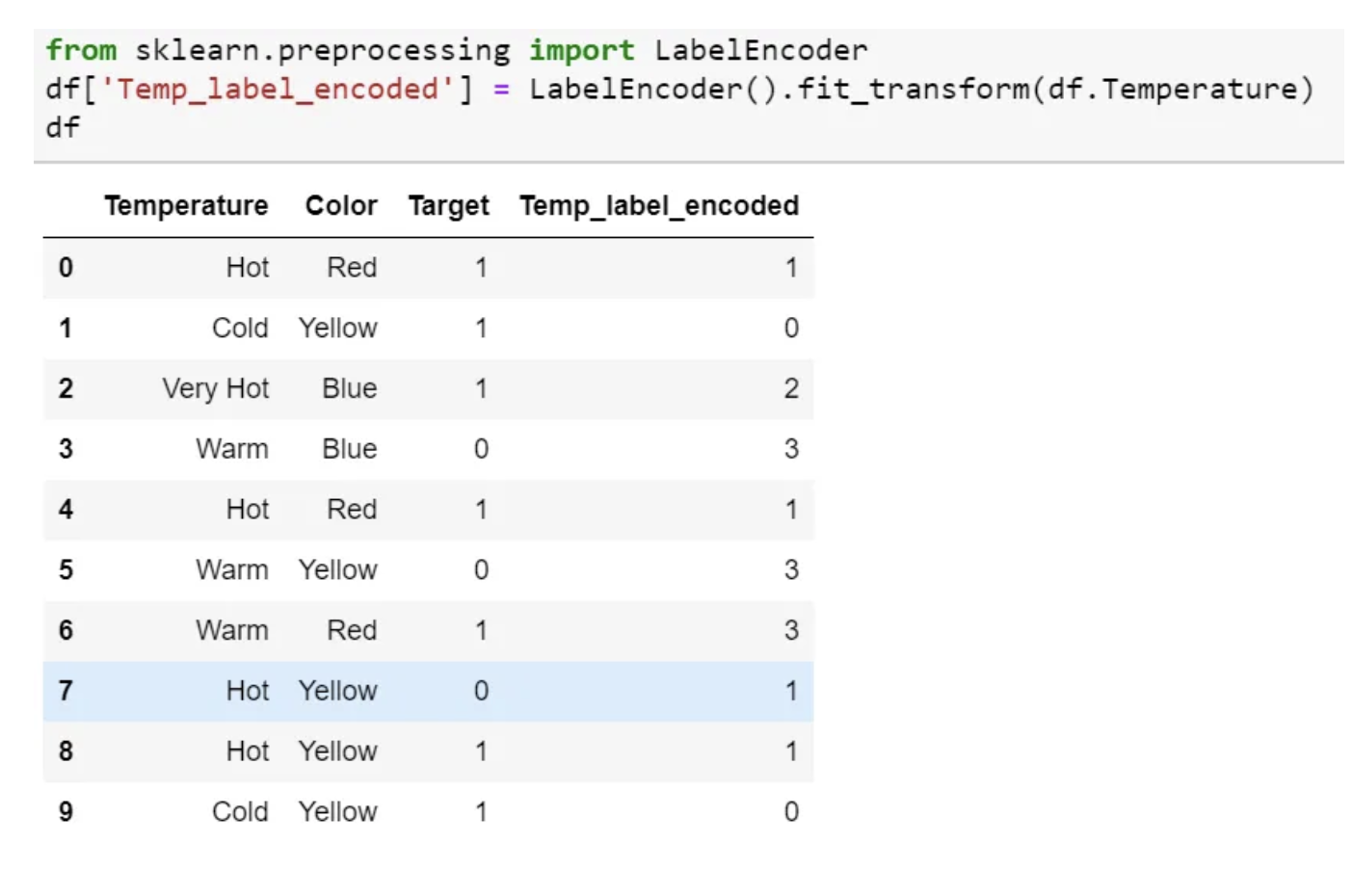
Label Encoding

• In this encoding, each category is assigned a value from 1 through N (where N is the number of categories for the feature.
• One major issue with this approach is there is no relation or order between these classes, but the algorithm might consider them as some order or some relationship.
• In below example it may look like (Cold<Hot<Very Hot<Warm….0 < 1 < 2 < 3 ).

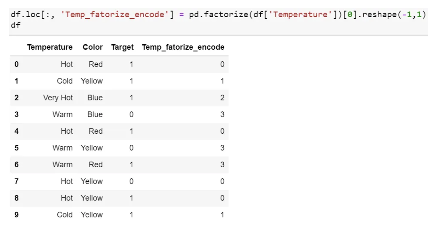
• Pandas factorize also perform the same function.

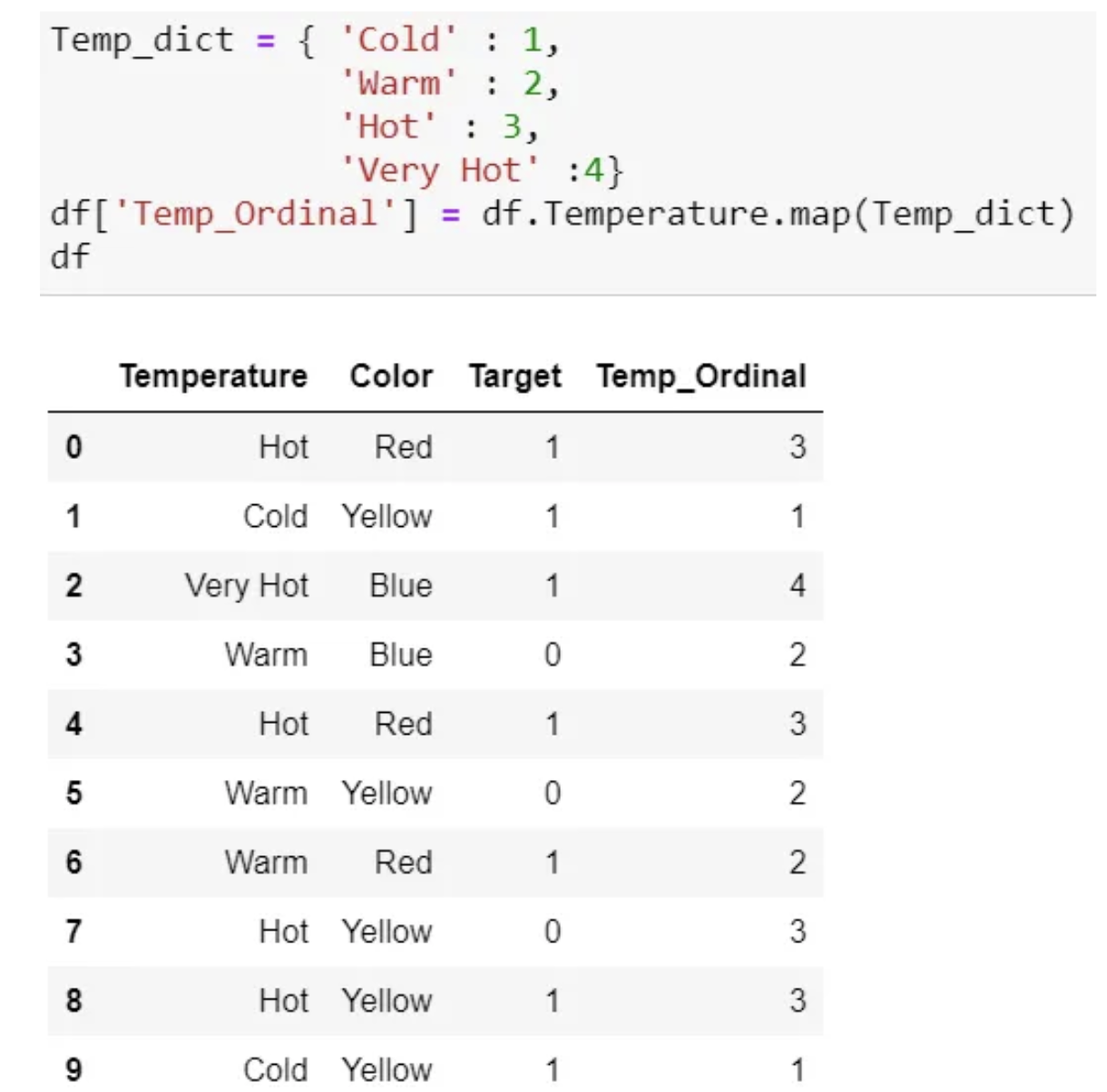
Ordinal Encoding

• This is reasonable only for ordinal variables.
• We do Ordinal encoding to ensure the encoding of variables retains the ordinal nature of the variable.
• slightly different as Label coding
  • as per the order of data (Pandas assigned Hot (0), Cold (1), “Very Hot” (2), and Warm (3)) or
  • as per alphabetically sorted order (scikit-learn assigned Cold(0), Hot(1), “Very Hot” (2), and Warm (3)).
• If we consider the temperature scale as the order, then the ordinal value should from cold to “Very Hot. “ Ordinal encoding will assign values as ( Cold(1) <Warm(2)<Hot(3)<”Very Hot(4)). Usually, Ordinal Encoding is done starting from 1.

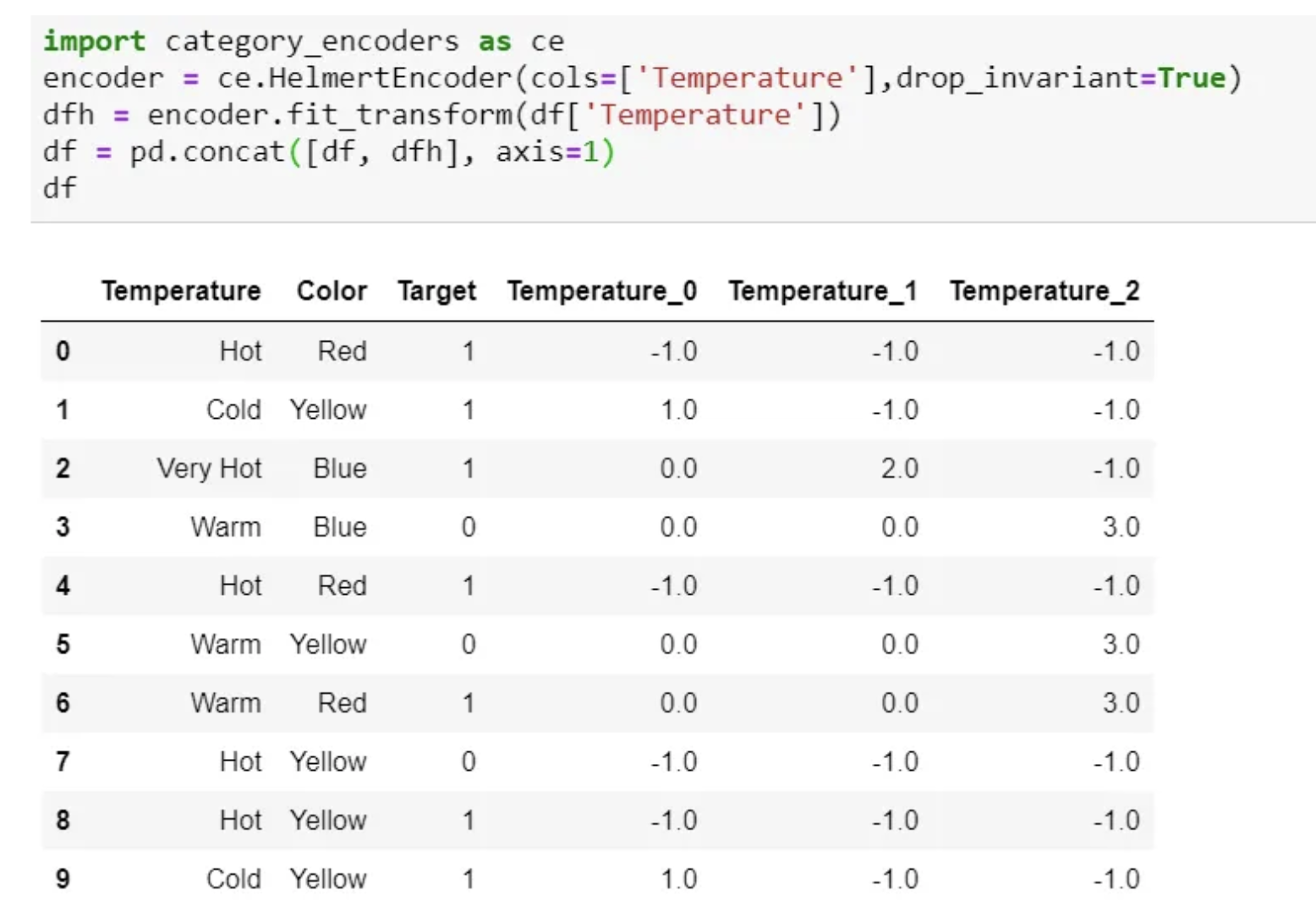
Helmert Encoding

• In this encoding, the mean of the dependent variable for a level is compared to the mean of the dependent variable over all previous levels.

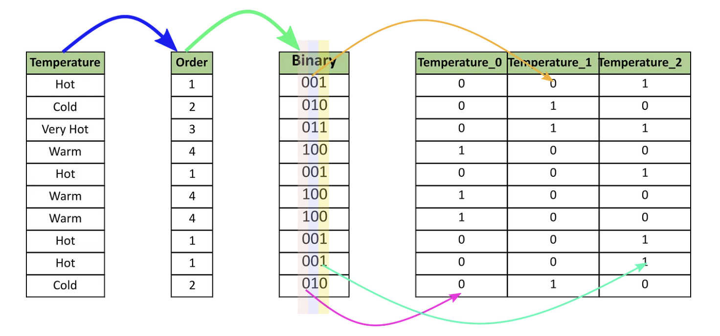
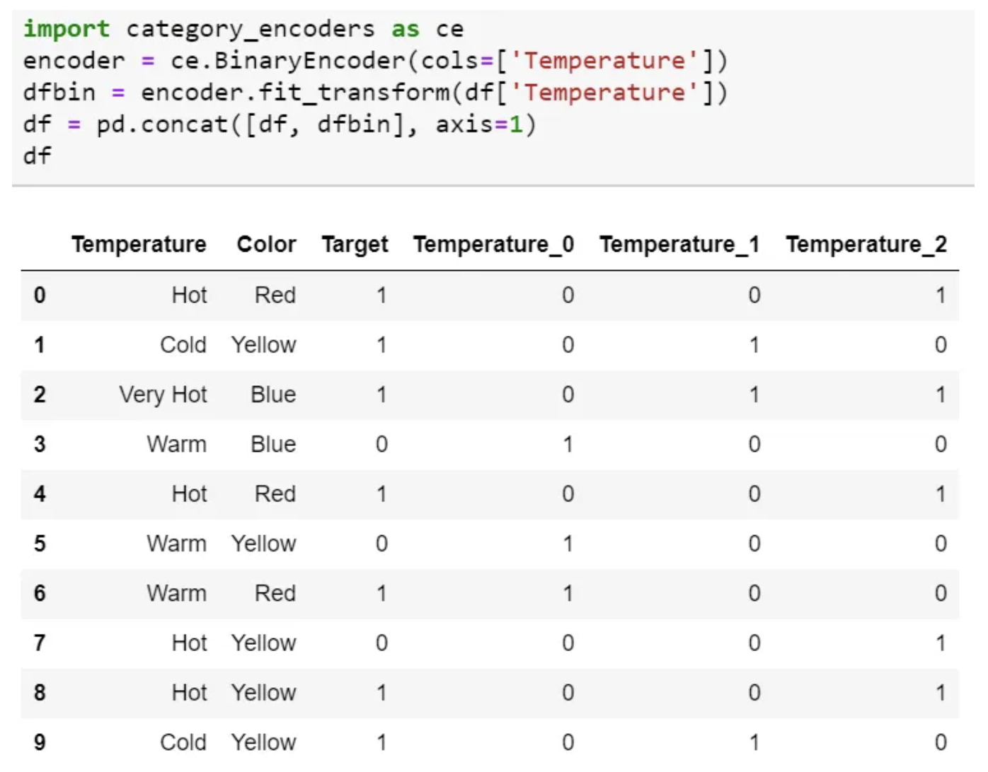
Binary Encoding

• Binary encoding converts a category into binary digits.
• Each binary digit creates one feature column.
• If there are n unique categories, then binary encoding results in only $log_2(n)$ features.
  • For 100 categories, One Hot Encoding will have 100 features, while Binary encoding will need just seven features.

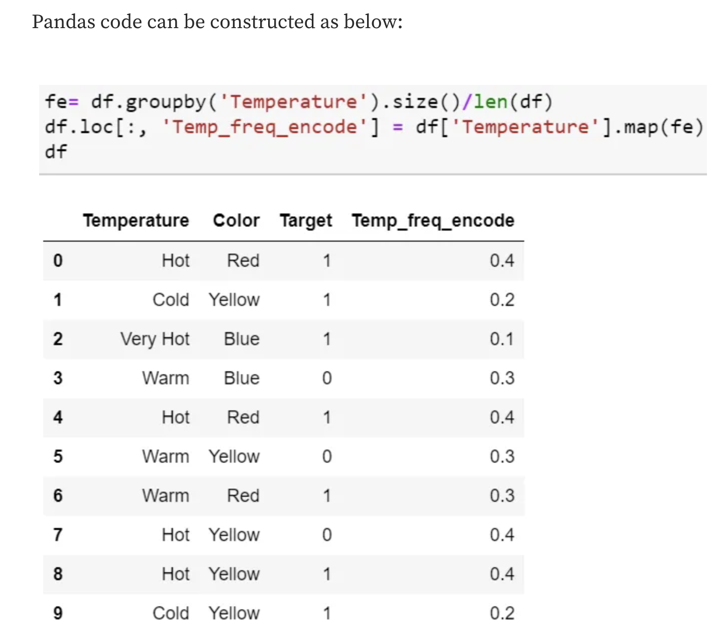
Frequency Encoding

• It is a way to utilize the frequency of the categories as labels.
• In the cases where the frequency is related somewhat to the target variable, it helps the model understand and assign the weight in direct and inverse proportion, depending on the nature of the data.

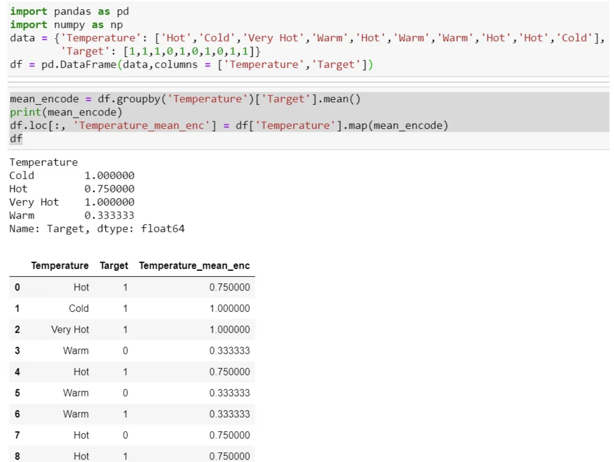
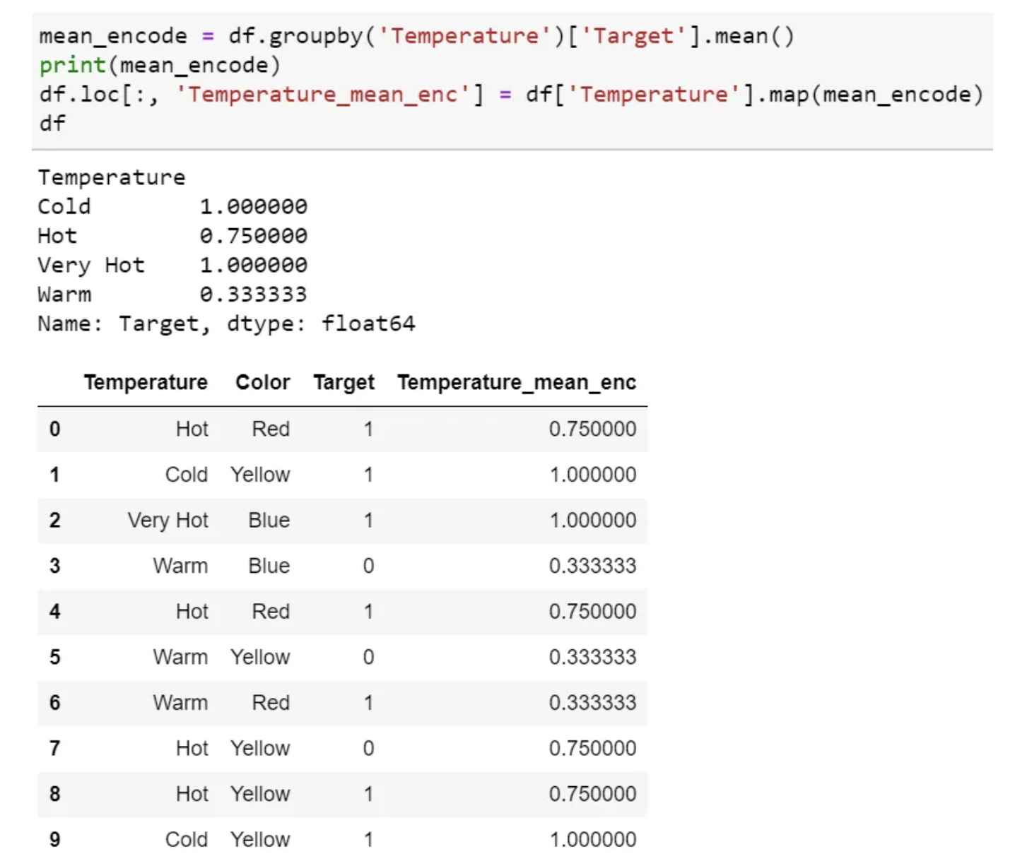
Mean Encoding

• Mean Encoding or Target Encoding is one viral encoding approach followed by Kagglers.
• There are many variations of this.
• Mean encoding is similar to label encoding, except here, labels are correlated directly with the target.
• This encoding method brings out the relation between similar categories, but the connections are bounded within the categories and the target itself.
• Pros: it does not affect the volume of the data and helps in faster learning.
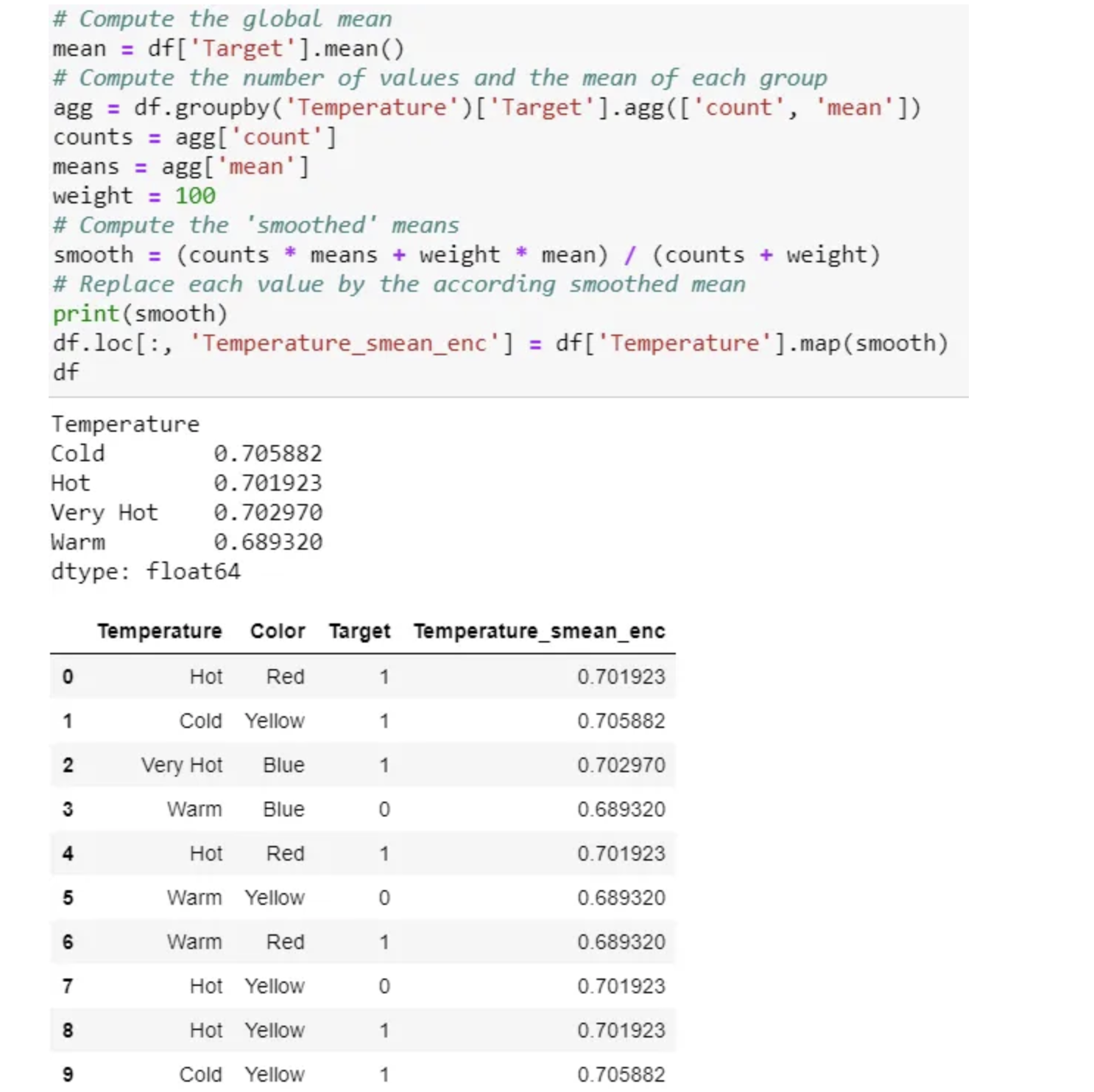
• Usually, Mean encoding is notorious for over-fitting; thus, a regularization with cross-validation or some other approach is a must on most occasions.

1. Select a categorical variable you would like to transform.
2. Group by the categorical variable and obtain aggregated sum over the “Target” variable. (total number of 1’s for each category in ‘Temperature’)
3. Group by the categorical variable and obtain aggregated count over “Target” variable
4. Divide the step 2 / step 3 results and join it back with the train.

• Mean encoding can embody the target in the label, whereas label encoding does not correlate with the target.
• In the case of many features, mean encoding could prove to be a much simpler alternative.
• Mean encoding tends to group the classes, whereas the grouping is random in label encoding.

There are many variations of this target encoding in practice, like smoothing. Smoothing can implement as below:

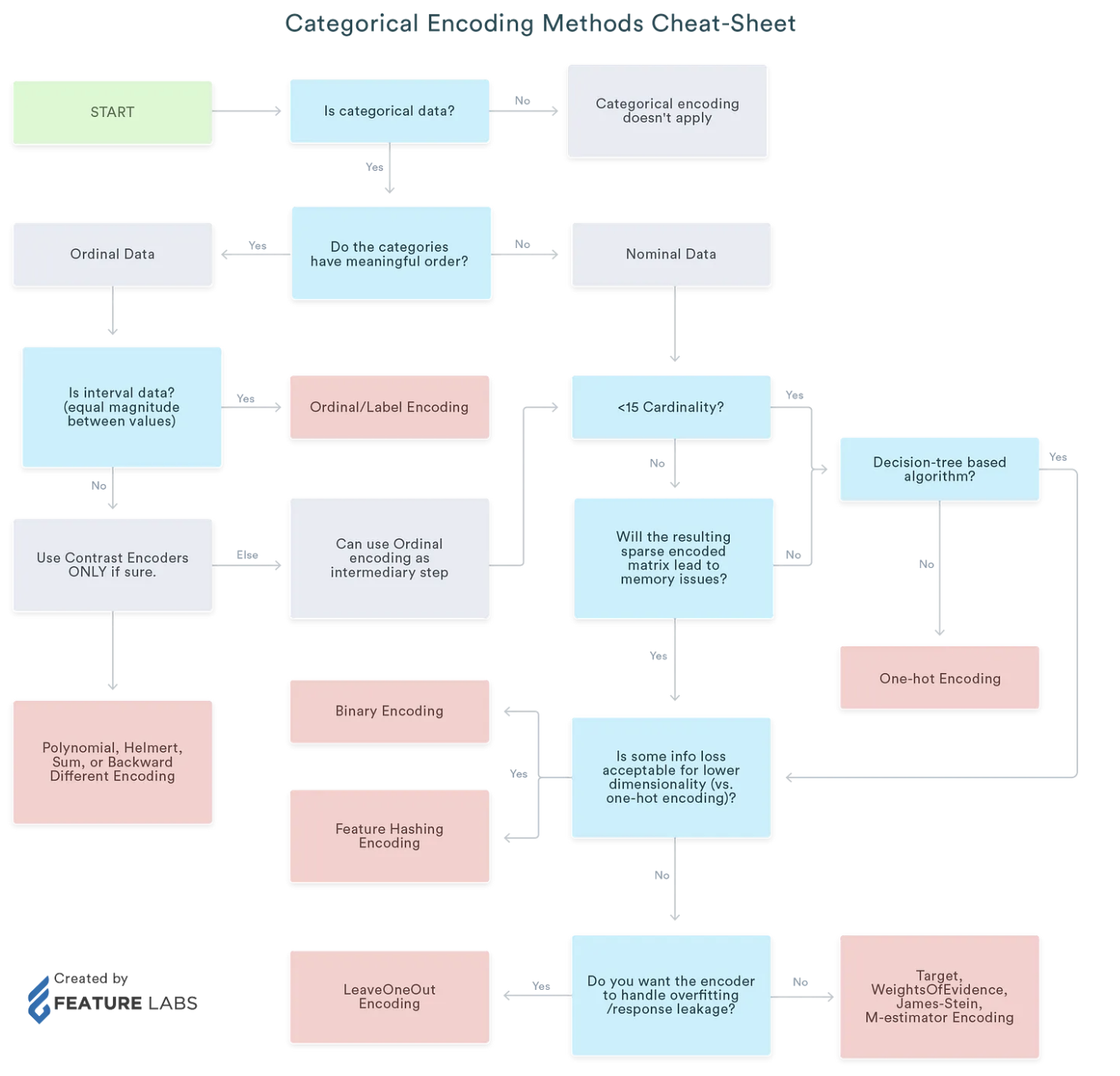
Summary of Categorical Encoding

Encoding for Quantitive variables

Binning

Linear models can only model linear relationships, which are lines in the case of a single feature. The decision tree can build a much more complex model of the data. However, this is strongly dependent on the representation of the data.

One way to make linear models more powerful on continuous data is to use binning (also known as discretization) of the feature to split it up into multiple features.

import mglearn
import matplotlib.pyplot as plt
from sklearn.linear_model import LinearRegression
from sklearn.tree import DecisionTreeRegressor

X, y = mglearn.datasets.make_wave(n_samples=100)
line = np.linspace(-3, 3, 1000, endpoint=False).reshape(-1, 1)
reg = DecisionTreeRegressor(min_samples_split=3).fit(X, y)
plt.plot(line, reg.predict(line), label="decision tree")
reg = LinearRegression().fit(X, y)

plt.plot(line, reg.predict(line), label="linear regression")
plt.plot(X[:, 0], y, 'o', c='k')
plt.ylabel("Regression output")
plt.xlabel("Input feature")
plt.legend(loc="best")

<matplotlib.legend.Legend at 0x7f886b901f40>

• We imagine a partition of the input range for the feature (in this case, the numbers from –3 to 3) into a fixed number of bins—say, 10.

• We create 11 entries, which will create 10 bins.

bins = np.linspace(-3, 3, 11)
print("bins: {}".format(bins))

bins: [-3.  -2.4 -1.8 -1.2 -0.6  0.   0.6  1.2  1.8  2.4  3. ]

which_bin = np.digitize(X, bins=bins)
print("\nData points:\n", X[:5])
print("\nBin membership for data points:\n", which_bin[:5])

Data points:
 [[-0.75275929]
 [ 2.70428584]
 [ 1.39196365]
 [ 0.59195091]
 [-2.06388816]]

Bin membership for data points:
 [[ 4]
 [10]
 [ 8]
 [ 6]
 [ 2]]

from sklearn.preprocessing import OneHotEncoder
# transform using the OneHotEncoder
encoder = OneHotEncoder(sparse=False)
# encoder.fit finds the unique values that appear in which_bin
encoder.fit(which_bin)
# transform creates the one-hot encoding
X_binned = encoder.transform(which_bin)
print(X_binned[:5])

#Because we specified 10 bins, the transformed dataset X_binned now is made up of 10 features.
print("X_binned.shape: {}".format(X_binned.shape))

[[0. 0. 0. 1. 0. 0. 0. 0. 0. 0.]
 [0. 0. 0. 0. 0. 0. 0. 0. 0. 1.]
 [0. 0. 0. 0. 0. 0. 0. 1. 0. 0.]
 [0. 0. 0. 0. 0. 1. 0. 0. 0. 0.]
 [0. 1. 0. 0. 0. 0. 0. 0. 0. 0.]]
X_binned.shape: (100, 10)

line_binned = encoder.transform(np.digitize(line, bins=bins))
reg = LinearRegression().fit(X_binned, y)
plt.plot(line, reg.predict(line_binned), label='linear regression binned')
reg = DecisionTreeRegressor(min_samples_split=3).fit(X_binned, y)
plt.plot(line, reg.predict(line_binned), label='decision tree binned')
plt.plot(X[:, 0], y, 'o', c='k')
plt.vlines(bins, -3, 3, linewidth=1, alpha=.2)
plt.legend(loc="best")
plt.ylabel("Regression output")
plt.xlabel("Input feature")

Text(0.5, 0, 'Input feature')

• The dashed line and solid line are exactly on top of each other, meaning the linear regression model and the decision tree make exactly the same predictions. For each bin, they predict a constant value.

• The linear model became much more flexible, because it now has a different value for each bin, while the decision tree model got much less flexible.

• The linear model benefited greatly in expressiveness from the transformation of the data.

• If the dataset is very large and high-dimensional, but some features have nonlinear relations, the binning can be a great way to increase modeling power.

1. Binning features generally has no beneficial effect for tree-based models, as these models can learn to split up the data anywhere. In a sense, that means decision trees can learn whatever binning is most useful

for predicting on this data. 2. decision trees look at multiple features at once, while binning is usually done on a per-feature basis.

Feature scaling

• In many machine learning algorithms, to bring all features in the same standing, we need to do scaling so that one significant number doesn’t impact the model just because of their large magnitude.
• Feature scaling in machine learning is one of the most critical steps during the pre-processing of data before creating a machine learning model.
• Like most other machine learning steps, feature scaling too is a trial and error process, not a single silver bullet.
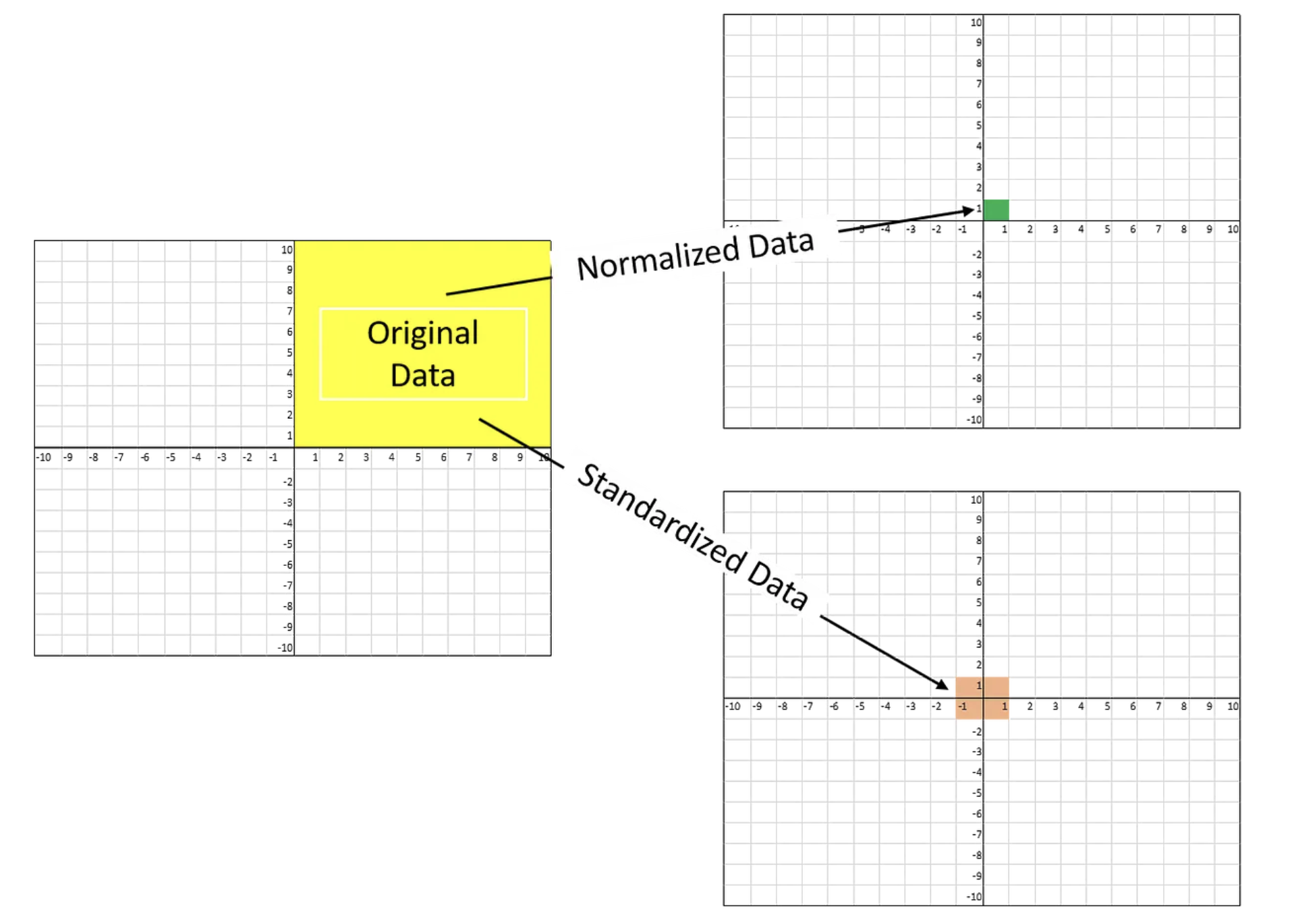
• The most common techniques of feature scaling are Normalization and Standardization.
  • Normalization is used when we want to bound our values between two numbers, typically, between [0,1] or [-1,1].
  • While Standardization transforms the data to have zero mean and a variance of 1, they make our data unitless.

Normalizer does a very different kind of rescaling. It scales each data point such that the feature vector has a Euclidean length of 1. In other words, it projects a data point on the circle (or sphere, in the case of higher dimensions) with a radius of 1.

• SVM, Linear Regression, Logistic Regression assume that data follow the Gaussian distribution.

• It is important to apply exactly the same transformation to the training set and the test set for the supervised model to work on the test set.

  • We call fit on the training set, and then call transform on the training and test sets.

Why need scaling?

The ML algorithm is sensitive to the “relative scales of features.

1. The feature with a higher value range dominants the other features.

• If there is a vast difference in the range, it makes the underlying assumption that higher ranging numbers have superiority of some sort.
• These more significant number starts playing a more decisive role while training the model.

• These more significant number of weights starts playing a more decisive role while training the model.
• Interestingly, if we convert the weight to “Kg,” then “Price” becomes dominant.

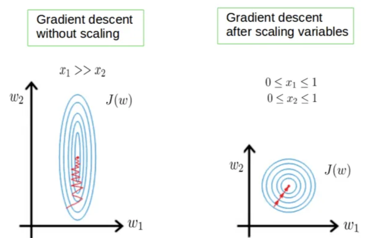
1. Few algorithms like Neural network gradient descent converge much faster with feature scaling than without it.

1. Saturation, like in the case of sigmoid activation in Neural Network, scaling would help not to saturate too fast.

When to do scaling?

Rule of thumb we may follow here is an algorithm that computes distance or assumes normality, scales your features.

Some examples of algorithms where feature scaling matters are:

• K-nearest neighbors (KNN) with a Euclidean distance measure is sensitive to magnitudes and hence should be scaled for all features to weigh in equally.
• K-Means uses the Euclidean distance measure here feature scaling matters.
• Scaling is critical while performing Principal Component Analysis(PCA). PCA tries to get the features with maximum variance, and the variance is high for high magnitude features and skews the PCA towards high magnitude features.
• We can speed up gradient descent by scaling because θ descends quickly on small ranges and slowly on large ranges, and oscillates inefficiently down to the optimum when the variables are very uneven.

Algorithms that do not require normalization/scaling are the ones that rely on rules. They would not be affected by any monotonic transformations of the variables. Scaling is a monotonic transformation.

• Examples of algorithms in this category are all the tree-based algorithms — CART, Random Forests, Gradient Boosted Decision Trees. These algorithms utilize rules (series of inequalities) and do not require normalization.

Algorithms like Linear Discriminant Analysis(LDA), Naive Bayes is by design equipped to handle this and give weights to the features accordingly. Performing features scaling in these algorithms may not have much effect.

MinMaxScaler (Normalization)

• All of the features are between 0 and 1.
• This Scaler shrinks the data within the range of -1 to 1 if there are negative values.
• This Scaler responds well if the standard deviation is small and when a distribution is not Gaussian.
• This Scaler is sensitive to outliers.

MinMaxScaler shifts the data such that all features are exactly between 0 and 1. For the two-dimensional dataset this means all of the data is contained within the rectangle created by the x-axis between 0 and 1 and the y-axis

between 0 and 1.

\(X_{std} = \frac{X - X_{min}}{X_{max} - X_{min}},\) and \(X_{scaled} = X_{std} * (max - min) + min.\)

where max, min represent feature ranges.

from sklearn.preprocessing import MinMaxScaler

scaler = MinMaxScaler()
scaler.fit(iris_df)
iris_scaled = scaler.transform(iris_df)

iris_df_scaled = pd.DataFrame(data = iris_scaled, columns =iris.feature_names)
print('Mins of the features:\n{}'.format(iris_df_scaled.min())) 
print('Maxes of the features:\n{}'.format(iris_df_scaled.max())) 

Mins of the features:
sepal length (cm)    0.0
sepal width (cm)     0.0
petal length (cm)    0.0
petal width (cm)     0.0
dtype: float64
Maxes of the features:
sepal length (cm)    1.0
sepal width (cm)     1.0
petal length (cm)    1.0
petal width (cm)     1.0
dtype: float64

from sklearn.datasets import load_breast_cancer
from sklearn.model_selection import train_test_split
cancer = load_breast_cancer()

from sklearn.svm import SVC
X_train, X_test, y_train, y_test = train_test_split(cancer.data, cancer.target, random_state=23)
svm = SVC(C=100)
svm.fit(X_train, y_train)
print("Test set accuracy: {:.2f}".format(svm.score(X_test, y_test)))

Test set accuracy: 0.94

# Preprocessing using 0-1 scaling

scaler = MinMaxScaler()
scaler.fit(X_train)

X_train_scaled = scaler.transform(X_train)
X_test_scaled = scaler.transform(X_test)

# learning an SVM on the scaled training data
svm.fit(X_train_scaled, y_train)

# scoring on the scaled test set/ The effect of scaling the data is quite significant.
print("Scaled test set accuracy: {:.2f}".format(svm.score(X_test_scaled, y_test)))

Scaled test set accuracy: 0.97

Unit Vector Scaler (Normalization)

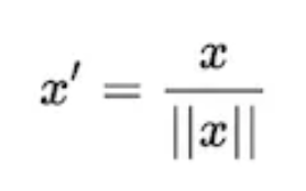
• Scaling is done considering the whole feature vector to be of unit length.
• Scaling to unit length shrinks/stretches a vector (a row of data can be viewed as a D-dimensional vector) to a unit sphere. When used on the entire dataset, the transformed data can be visualized as a bunch of vectors with different directions on the D-dimensional unit sphere.

This usually means dividing each component by the Euclidean length of the vector (L2 Norm). In some applications (e.g., histogram features), it can be more practical to use the L1 norm of the feature vector.

Like Min-Max Scaling, the Unit Vector technique produces values of range [0,1]. When dealing with features with hard boundaries, this is quite useful. For example, when dealing with image data, the colors can range from only 0 to 255.

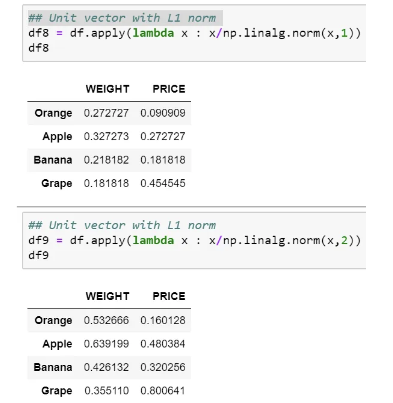
If we plot, then it would look as below for L1 and L2 norm, respectively.

StandardScaler

• The Standard Scaler assumes data is normally distributed within each feature and scales them such that the distribution centered around 0, with a standard deviation of 1.
• If data is not normally distributed, this is not the best Scaler to use.
• However, this scaling does not ensure any particular minimum and maximum values for the features.

import pandas as pd
from sklearn.datasets import load_iris
from sklearn.preprocessing import StandardScaler


iris = load_iris()
iris_df = pd.DataFrame(data = iris.data, columns = iris.feature_names)
print('Means of the features:\n{}'.format(iris_df.mean()))
print('Variances of the features:\n{}'.format(iris_df.var()))

Means of the features:
sepal length (cm)    5.843333
sepal width (cm)     3.057333
petal length (cm)    3.758000
petal width (cm)     1.199333
dtype: float64
Variances of the features:
sepal length (cm)    0.685694
sepal width (cm)     0.189979
petal length (cm)    3.116278
petal width (cm)     0.581006
dtype: float64

scaler = StandardScaler()
scaler.fit(iris_df)
iris_scaled = scaler.transform(iris_df) #NumPy ndarray

iris_df_scaled = pd.DataFrame(data = iris_scaled, columns = iris.feature_names)
print('Means of the features:\n{}'.format(iris_df_scaled.mean())) # All means are 0.
print('Variances of the features:\n{}'.format(iris_df_scaled.var())) # All variances are 1.

Means of the features:
sepal length (cm)   -1.690315e-15
sepal width (cm)    -1.842970e-15
petal length (cm)   -1.698641e-15
petal width (cm)    -1.409243e-15
dtype: float64
Variances of the features:
sepal length (cm)    1.006711
sepal width (cm)     1.006711
petal length (cm)    1.006711
petal width (cm)     1.006711
dtype: float64

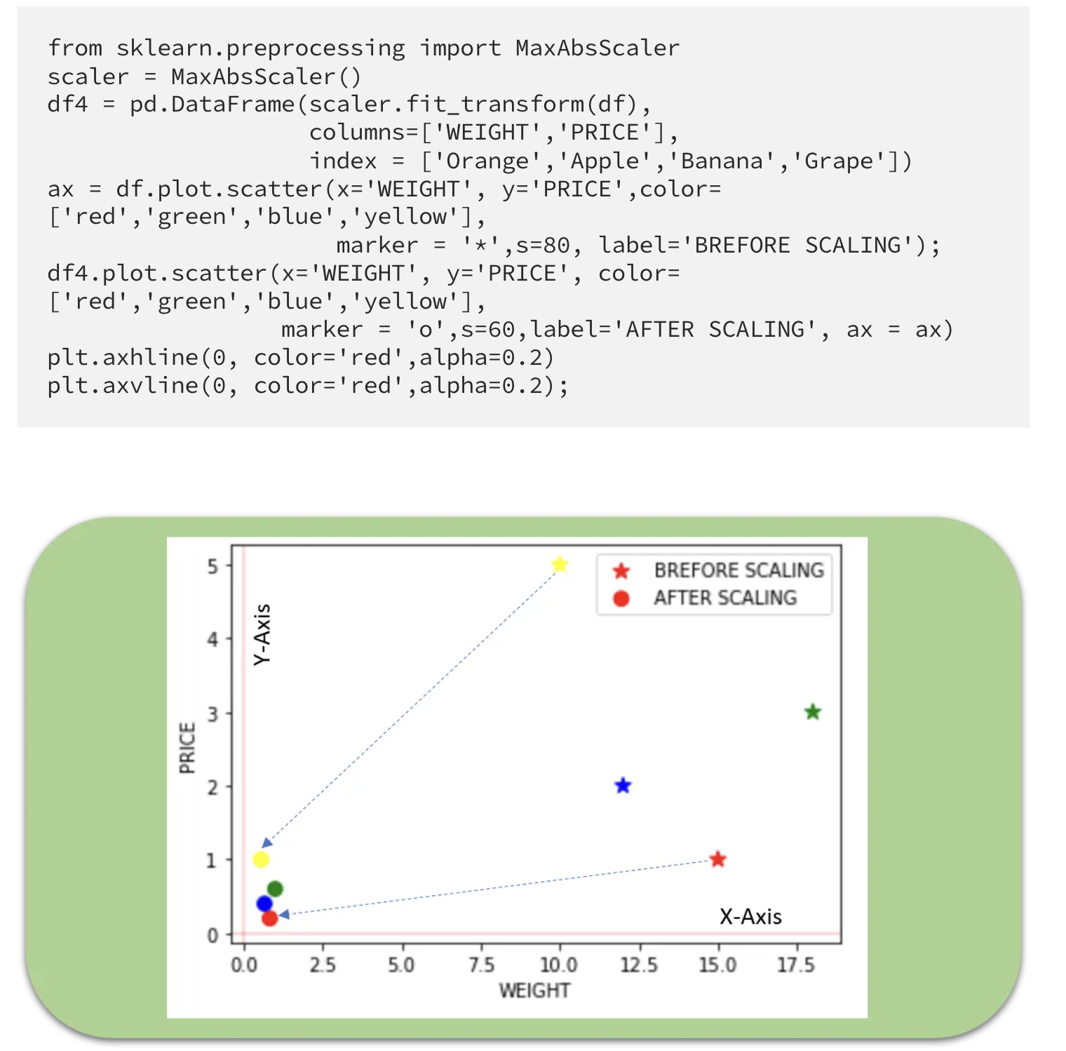
Max Abs Scaler

• Scale each feature by its maximum absolute value.
• This estimator scales and translates each feature individually such that the maximal absolute value of each feature in the training set is 1.0.
• It does not shift/center the data and thus does not destroy any sparsity.
• Cons: On positive-only data, this Scaler behaves similarly to Min Max Scaler and, therefore, also suffers from the presence of significant outliers.

Robust Scaler

• This Scaler is robust to outliers.
• If our data contains many outliers, scaling using the mean and standard deviation of the data won’t work well.
• The centering and scaling statistics of this Scaler are based on percentiles and are therefore not influenced by a few numbers of huge marginal outliers (The RobustScaler ignore outliers.).
• Note that the outliers themselves are still present in the transformed data. If a separate outlier clipping is desirable, a non-linear transformation is required.

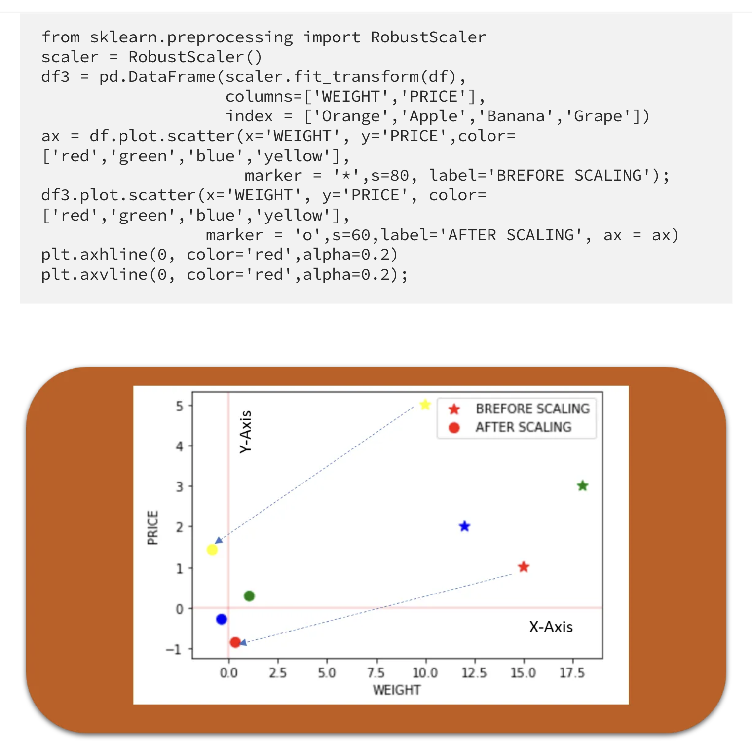
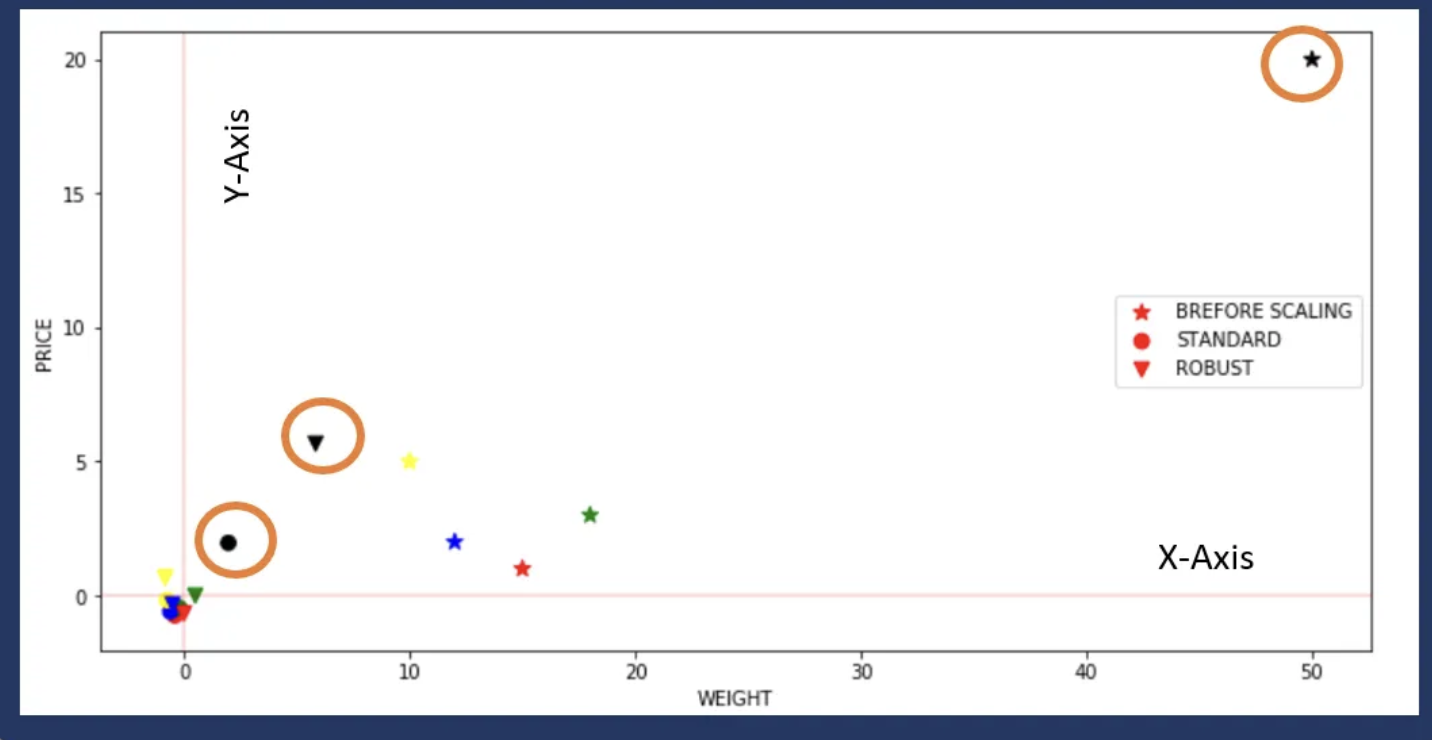
Let’s now see what happens if we introduce an outlier and see the effect of scaling using Standard Scaler and Robust Scaler (a circle shows outlier).

Quantile Transformer Scaler (Rank scaler)

• Transform features using quantiles information.
• This method transforms the features to follow a uniform or a normal distribution.
• Therefore, for a given feature, this transformation tends to spread out the most frequent values.
• It also reduces the impact of (marginal) outliers: this is, therefore, a robust pre-processing scheme.
• The cumulative distribution function of a feature is used to project the original values.
• Note that this transform is non-linear and may distort linear correlations between variables measured at the same scale but renders variables measured at different scales more directly comparable.

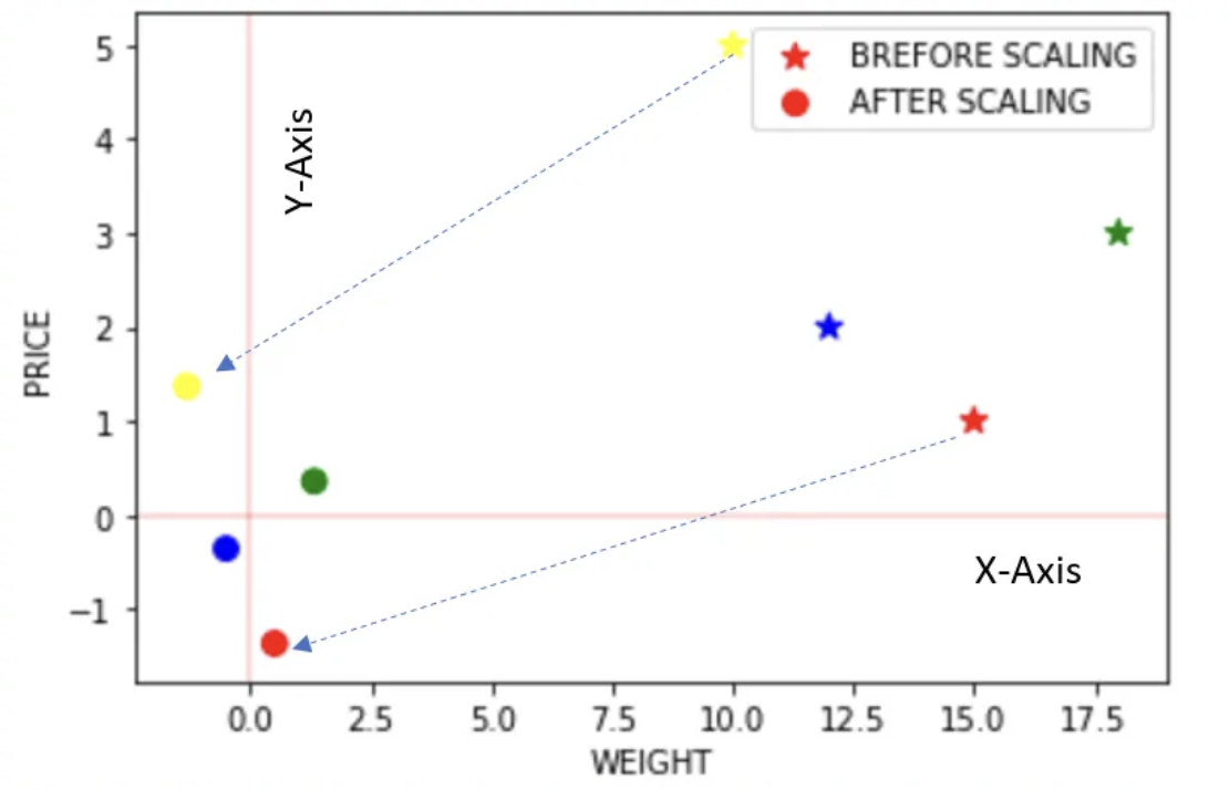
from sklearn.preprocessing import QuantileTransformer
scaler = QuantileTransformer()
df6 = pd.DataFrame(scaler.fit_transform(df),
                   columns=['WEIGHT','PRICE'],
                   index = ['Orange','Apple','Banana','Grape'])
ax = df.plot.scatter(x='WEIGHT', y='PRICE',color=['red','green','blue','yellow'], 
                     marker = '*',s=80, label='BREFORE SCALING');
df6.plot.scatter(x='WEIGHT', y='PRICE', color=['red','green','blue','yellow'],
                 marker = 'o',s=60,label='AFTER SCALING', ax = ax,figsize=(6,4))
plt.axhline(0, color='red',alpha=0.2)
plt.axvline(0, color='red',alpha=0.2);

The above example is just for illustration as Quantile transformer is useful when we have a large dataset with many data points usually more than 1000.

Power Transformer Scaler

• The power transformer is a family of parametric, monotonic transformations that are applied to make data more Gaussian-like.
• This is useful for modeling issues related to the variability of a variable that is unequal across the range (heteroscedasticity) or situations where normality is desired.
• The power transform finds the optimal scaling factor in stabilizing variance and minimizing skewness through maximum likelihood estimation.
• Currently, Sklearn implementation of PowerTransformer supports the Box-Cox transform and the Yeo-Johnson transform.
• The optimal parameter for stabilizing variance and minimizing skewness is estimated through maximum likelihood.
• Box-Cox requires input data to be strictly positive, while Yeo-Johnson supports both positive or negative data.

from sklearn.preprocessing import PowerTransformer
scaler = PowerTransformer(method='yeo-johnson')
df5 = pd.DataFrame(scaler.fit_transform(df),
                   columns=['WEIGHT','PRICE'],
                   index = ['Orange','Apple','Banana','Grape'])
ax = df.plot.scatter(x='WEIGHT', y='PRICE',color=['red','green','blue','yellow'], 
                     marker = '*',s=80, label='BREFORE SCALING');
df5.plot.scatter(x='WEIGHT', y='PRICE', color=['red','green','blue','yellow'],
                 marker = 'o',s=60,label='AFTER SCALING', ax = ax)
plt.axhline(0, color='red',alpha=0.2)
plt.axvline(0, color='red',alpha=0.2);

References

1. Encoding
2. Scaling