Cross-Validation (CV)

Train/ Test split

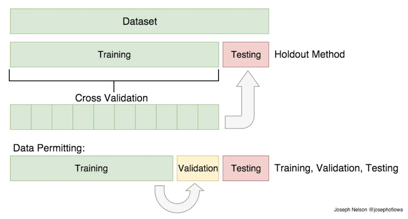
To evaluate our supervised models, we split our dataset into a training set and a test set and fit our model on the training set in order to make predictions on the test set using the scoring method.

• We are interested in how well our model can predict new data that was not trained.

from sklearn.datasets import load_iris
from sklearn.linear_model import LogisticRegression
from sklearn.model_selection import train_test_split
import warnings
warnings.filterwarnings('ignore')

iris_dataset = load_iris()

# Keys
print("Keys of iris_dataset: \n{}".format(iris_dataset.keys()))

# Feature_names: A list of the descriptions of features
print("Feature names: \n{}".format(iris_dataset['feature_names'])) 

# Shape of the data array X(n: 150, p: 4)
print("Shape of data: {}".format(iris_dataset['data'].shape))

# Target y: 0 means setosa, 1 means versicolor, and 2 means virginica.
print("Target:\n{}".format(iris_dataset['target']))

X_train, X_test, y_train, y_test = train_test_split(iris_dataset['data'], iris_dataset['target'], test_size = 0.2, random_state=12, shuffle=True) #A fixed seed:  If we want the splits to be reproducible, 

Keys of iris_dataset: 
dict_keys(['data', 'target', 'frame', 'target_names', 'DESCR', 'feature_names', 'filename', 'data_module'])
Feature names: 
['sepal length (cm)', 'sepal width (cm)', 'petal length (cm)', 'petal width (cm)']
Shape of data: (150, 4)
Target:
[0 0 0 0 0 0 0 0 0 0 0 0 0 0 0 0 0 0 0 0 0 0 0 0 0 0 0 0 0 0 0 0 0 0 0 0 0
 0 0 0 0 0 0 0 0 0 0 0 0 0 1 1 1 1 1 1 1 1 1 1 1 1 1 1 1 1 1 1 1 1 1 1 1 1
 1 1 1 1 1 1 1 1 1 1 1 1 1 1 1 1 1 1 1 1 1 1 1 1 1 1 2 2 2 2 2 2 2 2 2 2 2
 2 2 2 2 2 2 2 2 2 2 2 2 2 2 2 2 2 2 2 2 2 2 2 2 2 2 2 2 2 2 2 2 2 2 2 2 2
 2 2]

• Before splitting, the train_test_split function shuffles the dataset using a pseudorandom number generator.

• It extracts 75% of the rows in the data as the training set and the remaining 25% of the data as the test set.

# Instantiate a model and fit it to the training set
logreg = LogisticRegression().fit(X_train, y_train)
# evaluate the model on the test set
print("Test set score: {:.2f}".format(logreg.score(X_test, y_test)))

Test set score: 0.97

But train/test split does have its dangers

• what if the split we make isn’t random?
• What if one subset of our data has only people from a certain state, employees with a certain income level but not other income levels, only women, or only people at a certain age? (imagine a file ordered by one of these).
• This will result in overfitting, even though we’re trying to avoid it! This is where cross-validation comes in.

For a better estimate of the generalization performance, instead of using a single split into a training and a validation set, we can use cross-validation to evaluate the performance of each parameter combination.

Cross-Validation

• Cross-validation is a statistical method of evaluating generalization performance that is more stable and thorough than using a split into a training and a test set.

• When performing five-fold cross-validation, we split our data into k subsets, and train on k-1 one of those subsets.

• The first model is trained using the first fold as the test set, and the remaining folds (2–5) are used as the training set.

• The model is built using the data in folds 2–5; the accuracy is evaluated on fold 1.

• Benefits

  • When using cross-validation, each example will be in the test set exactly once: each example is in one of the folds, and each fold is the test set once. On the other hand, train_test_split performs a random split of the data.

  • We use our data more effectively. When using 10-fold cross-validation, we can use nine-tenths of the data (90%) to fit the model. More data will usually result in more accurate models.

• Disadvantage
  • Increased computational cost: Roughly $k$ times slower than doing a single split of the data.

import numpy as np
from sklearn.datasets import load_iris
from sklearn.linear_model import LogisticRegression
from sklearn.model_selection import cross_val_score

iris_dataset = load_iris()
logreg = LogisticRegression()
scores = cross_val_score(logreg, iris.data, iris.target, cv= 5) #Function, X, y
print("Cross-validation scores: {}".format( np.round(scores, 3)))
# Compute the mean to summarize the cross-validation accuracy.
print("Average cross-validation score: {:.2f}".format(scores.mean()))

Cross-validation scores: [0.967 1.    0.933 0.967 1.   ]
Average cross-validation score: 0.97

• Cross_val_score takes the dataset and applies cross-validation to split the data. Then, train a model using the specified estimator (e.g., logistic regression, decision tree, …) and measure the performance of the model (scoring parameter).

• Using the mean cross-validation, we can conclude that we expect the model to be around 97% accurate on average.

• There is a relatively high variance in the accuracy between folds, ranging from 100% accuracy to 93% accuracy.

  • The model is very dependent on the particular folds used for training because of the small size of the dataset.

How many folds?

• The more folds we have, we will reduce the error due to the bias but increase the error due to variance.
• The computational price would go up too. The more folds you have, the longer it would take to compute it, and you would need more memory.
• With a lower number of folds, we’re reducing the error due to variance, but the error due to bias would be bigger. It’s would also computationally cheaper.
• In big datasets, k=3 is usually advised. In smaller datasets, as I’ve mentioned before, it’s best to use LOOCV.

Leave One Out Cross Validation (LOOCV)

• In this type of cross-validation, the number of folds (subsets) equals the number of observations we have in the dataset.
• We only use one data point for testing and the remaining data points for training.
• We then average ALL of these folds and build our model with the average. We then test the model against the last fold.
• Because we would get a large number of training sets (equal to the number of samples), this method is very computationally expensive and should be used on small datasets.

from sklearn.model_selection import LeaveOneOut 
X = np.array([[1, 2], [3, 4]])
y = np.array([1, 2])
loo = LeaveOneOut()
loo.get_n_splits(X)


for train_index, test_index in loo.split(X):
   print("TRAIN:", train_index, "TEST:", test_index)
   X_train, X_test = X[train_index], X[test_index]
   y_train, y_test = y[train_index], y[test_index]
   print(X_train, X_test, y_train, y_test)

('TRAIN:', array([1]), 'TEST:', array([0]))
(array([[3, 4]]), array([[1, 2]]), array([2]), array([1]))
('TRAIN:', array([0]), 'TEST:', array([1]))
(array([[1, 2]]), array([[3, 4]]), array([1]), array([2]))

Stratified k-fold CV

• Splitting the dataset into k folds by starting with the first one-k-th part of the data might not always be a good idea.

  • In classification tasks with imbalanced class distributions, we should prefer StratifiedKFold over KFold.

  • What if the test set would be only class 0, and the training set would be only classes 1 and 2? As the classes in training and test sets would be different for all three splits, the three-fold cross-validation accuracy would be zero on this dataset.

  • If 90% of your samples belong to class A and 10% of your samples belong to class B, then stratified cross-validation ensures that in each fold, 90% of samples belong to class A and 10% of samples belong to class B.

• Scikit-learn does not use it for classification but rather uses stratified k-fold cross-validation.

• For regression, Scikit-learn uses the standard k-fold cross-validation by default.

CV with groups

• When there are groups in the data that are highly related, it is commonly used.

• GroupKFold is a variation of k-fold that ensures that the same group is not represented in both testing and training sets.

• Say you want to build a system to recognize emotions from pictures of faces, and you collect a dataset of pictures of 100 people where each person is captured multiple times, showing various emotions.

• It is likely that pictures of the same person will be in both the training and the test set.

• To accurately evaluate the generalization to new faces, we must therefore ensure that the training and test sets contain images of different people.

from sklearn.model_selection import GroupKFold

X = [0.1, 0.2, 2.2, 2.4, 2.3, 4.55, 5.8, 8.8, 9, 10]
y = ["a", "b", "b", "b", "c", "c", "c", "d", "d", "d"]
groups = [1, 1, 1, 2, 2, 2, 3, 3, 3, 3]

gkf = GroupKFold(n_splits=3)
for train, test in gkf.split(X, y, groups=groups):
    print("%s %s" % (train, test))

[0 1 2 3 4 5] [6 7 8 9]
[0 1 2 6 7 8 9] [3 4 5]
[3 4 5 6 7 8 9] [0 1 2]

Grid Search

import pandas as pd
import mglearn
from sklearn.datasets import load_iris
from sklearn.tree import DecisionTreeClassifier
from sklearn.model_selection import GridSearchCV

iris_dataset = load_iris()
X_train, X_test, y_train, y_test = train_test_split(iris_dataset.data, iris_dataset.target, test_size = 0.2, random_state= 12)

dtree = DecisionTreeClassifier()

#Specify the parameters you want to search over using a dictionary.
param_grid = {'max_depth':[1, 2, 3], 'min_samples_split':[2, 3, 6]}

#Instantiate the GridSearchCV class with the model, the parameter grid, and cv strategy.
grid_dtree = GridSearchCV(dtree, param_grid, cv=5, refit = True) #refit = True: Default

#Fit a new model on the training dataset with the parameters.
grid_dtree.fit(X_train, y_train)

results_df = pd.DataFrame(grid_dtree.cv_results_)
print(results_df[ ['params', 'mean_test_score', 'rank_test_score'] ] )

scores = np.array(results_df.mean_test_score).reshape(3, 3)

# Plot the mean cross-validation scores
mglearn.tools.heatmap(scores, xlabel='max_depth', xticklabels=param_grid['max_depth'],
ylabel='min_samples_split', yticklabels=param_grid['min_samples_split'], cmap="viridis")

                                     params  mean_test_score  rank_test_score
0  {'max_depth': 1, 'min_samples_split': 2}         0.625000                7
1  {'max_depth': 1, 'min_samples_split': 3}         0.625000                7
2  {'max_depth': 1, 'min_samples_split': 6}         0.625000                7
3  {'max_depth': 2, 'min_samples_split': 2}         0.908333                4
4  {'max_depth': 2, 'min_samples_split': 3}         0.908333                4
5  {'max_depth': 2, 'min_samples_split': 6}         0.908333                4
6  {'max_depth': 3, 'min_samples_split': 2}         0.950000                1
7  {'max_depth': 3, 'min_samples_split': 3}         0.950000                1
8  {'max_depth': 3, 'min_samples_split': 6}         0.950000                1

</pre>

• The min_samples_split parameter is searching over interesting values, but the max_dept parameter is not—or it could mean the max_dept parameter is not important.

#To evaluate how well the best found parameters generalize, we can call score on the test set.
print("Best parameters: {}".format(grid_dtree.best_params_))
print("Best cross-validation score: {:.2f}".format(grid_dtree.best_score_))
print("Test set score: {:.2f}".format(grid_dtree.score(X_test, y_test)))

Best parameters: {'max_depth': 3, 'min_samples_split': 2}
Best cross-validation score: 0.95
Test set score: 0.93