
Bias-Variance Tradeoff
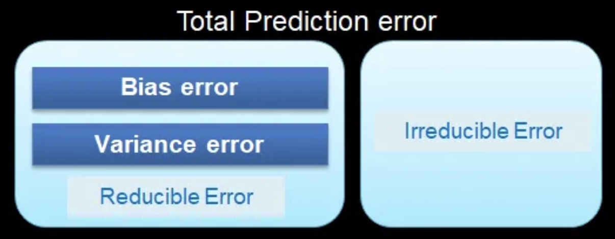
Whenever we build a prediction model, even after all the adjustments and treatments, our predictions will generally be imperfect: there will be some nonzero difference between the predicted and the actual values. This difference is called prediction error. We can decompose prediction error into two components: Reducible and Irreducible error.
Bias: The difference between the average prediction of our model and the correct value which we are trying to predict.
-
High bias: little attention to the training data and oversimplifies the model. -
A model has low number of predictors.
-
It leads to high errors in training and test data.
Variance: The variability of model prediction for a given data point or a value that tells us the spread of our data.
-
High variance: pays a lot of attention to training data and does not generalize on the data which it hasn’t seen before. -
The model is highly sensitive to small fluctuations and has a very large number of predictors. -> A very Complex model.
-
4It performs very well on training data but has high error rates on test data.
Math
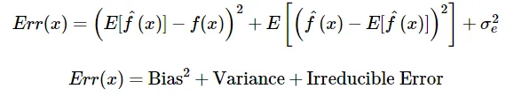
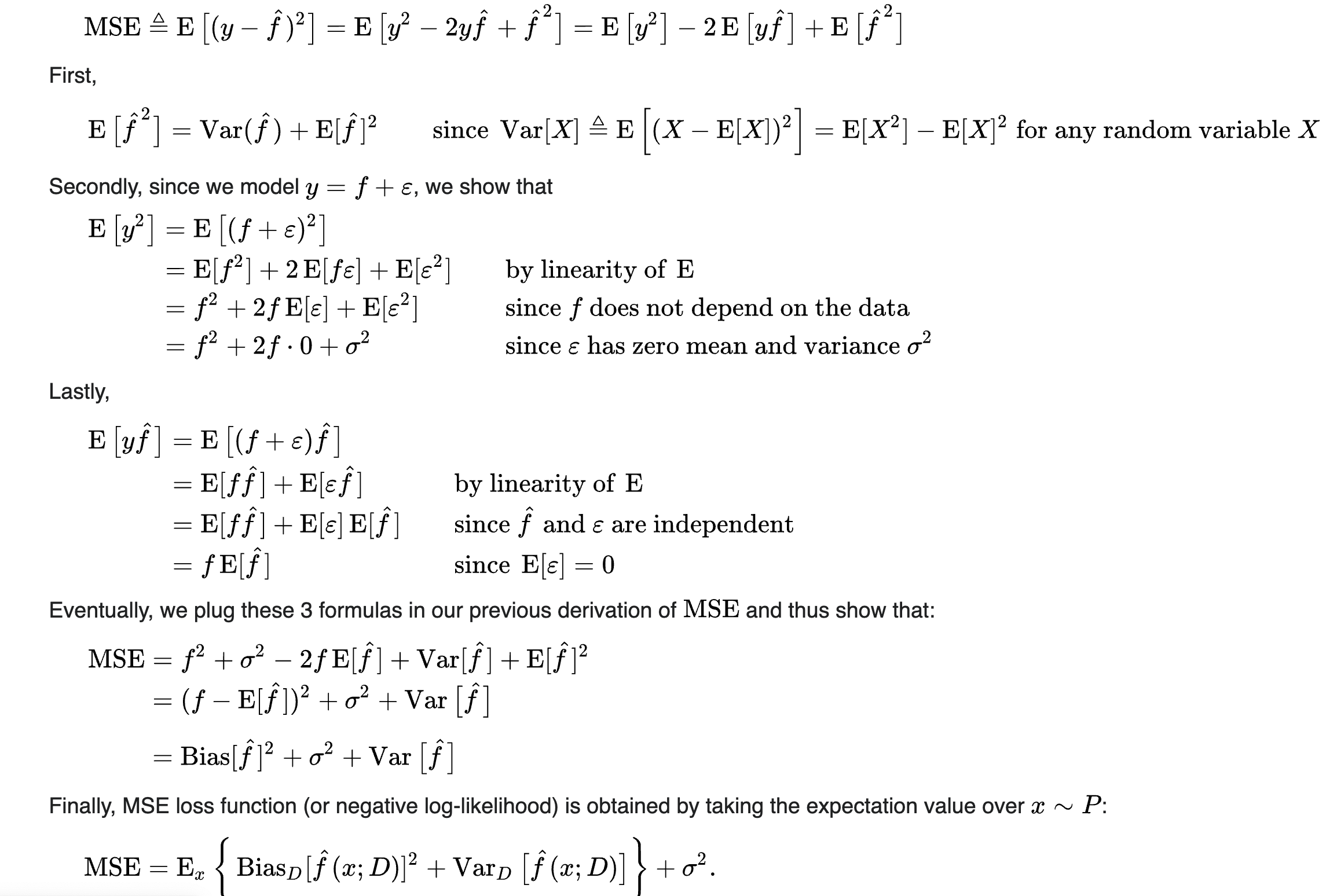
Let the variable we are trying to predict as Y and other covariates as X. We assume there is a relationship between the two such that $Y=f(X) + e$. Then the expected squared error at a point x is 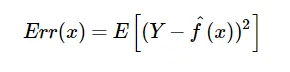
Then,
Irreducible error is an error that can’t be reduced by creating good models. It is a measure of the amount of noise in our data.
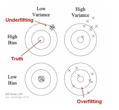
Overfitting and underfitting
Underfitting happens when a model unable to capture the underlying pattern of the data.
-
High bias and low variance -
When we have very little data to build an accurate model or try to build a linear model with nonlinear data.
-
Models are very
simpleto capture the complex patterns
Overfitting happens when our model captures the noise along with the underlying pattern in data.
-
Low bias and high variance -
It happens when we train our model a lot over noisy datasets.
-
These models are very complex, like Decision trees which are prone to overfitting.
Overfitting in Polynomial Regression
import numpy as np
import matplotlib.pyplot as plt
from sklearn.pipeline import Pipeline
from sklearn.preprocessing import PolynomialFeatures
from sklearn.linear_model import LinearRegression
from sklearn.model_selection import cross_val_score
%matplotlib inline
def true_fun(X):
    return np.cos(1.5*np.pi*X)

np.random.seed(0)
n =30
X = np.sort(np.random.rand(n))

y = true_fun(X) + np.random.randn(n)*0.1
We model the regression with degree 1, 4, and 15.
plt.figure(figsize=(14,5))
degrees = [1,4,15]

for i in range(len(degrees)):
    ax = plt.subplot(1, len(degrees), i+1)
    plt.setp(ax, xticks=(), yticks=())

    polynomial_features=PolynomialFeatures(degree=degrees[i], include_bias=False)

    pipeline = Pipeline([('poly', polynomial_features),('linear',LinearRegression())])
    pipeline.fit(X.reshape(-1,1), y) # reshape(-1,1) : one column

    scores = cross_val_score(pipeline, X.reshape(-1,1),y, scoring="neg_mean_squared_error", cv=10)
    coefficients = pipeline.named_steps['linear'].coef_
    print('\nDegree {0} coefficient is {1}.'.format(degrees[i], np.round(coefficients,2)))
    print('\nDegree {0} mse is {1}.'.format(degrees[i], -1*np.mean(scores)))


    X_test = np.linspace(0,1,100)

    plt.plot(X_test, pipeline.predict(X_test[:,np.newaxis]), label="Model")
    #X_test[:,np.newaxis], convert an 1D array to either a row vector or a column vector.
    #X_test.shape : (100,) , X_test[:,np.newaxis].shape : (100, 1)

    plt.plot(X_test,true_fun(X_test),'--', label="True function")
    plt.scatter(X, y, edgecolor='b', s=20, label="Samples")

    plt.xlabel("x"); plt.ylabel("y"); plt.xlim((0,1)); plt.ylim((-2,2)); plt.legend(loc="best")
    plt.title("Degree {0}\nMSE ={1:.2e}(+/- {2:.2e})".format(degrees[i], -scores.mean(), scores.std()))

plt.show()
Degree 1 coefficient is [-1.61].

Degree 1 mse is 0.40772896250986834.

Degree 4 coefficient is [  0.47 -17.79  23.59  -7.26].

Degree 4 mse is 0.04320874987231818.

Degree 15 coefficient is [-2.98295000e+03  1.03900050e+05 -1.87417308e+06  2.03717524e+07
 -1.44874234e+08  7.09320168e+08 -2.47067524e+09  6.24565587e+09
 -1.15677381e+10  1.56896159e+10 -1.54007266e+10  1.06458152e+10
 -4.91381762e+09  1.35920853e+09 -1.70382347e+08].

Degree 15 mse is 181777900.28556666.

The best degree is 4 where its MSE is the smallest value, 0.0432.
-
degree = 1, too simple model and too biased. High bias/ low variance.
-
degree=15 overfitting. Low bias/ High variance.
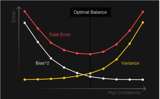
Bias-variance tradeoff
To build a good model, we need to find a good balance between bias and variance such that it minimizes the total error.
Total error = Bias^2 + Variance + Irreducible error
Leave a comment