Kaggle- Creditcard_Fraud_Detection
It is important that credit card companies are able to recognize fraudulent credit card transactions so that customers are not charged for items that they did not purchase.
The dataset contains transactions made by credit cards in September 2013 by European cardholders. This dataset presents transactions that occurred in two days, where we have 492 frauds out of 284,807 transactions. The dataset is highly unbalanced, the positive class (frauds) account for 0.172% of all transactions.
It contains only numerical input variables which are the result of a PCA transformation. Features V1, V2, … V28 are the principal components obtained with PCA, the only features which have not been transformed with PCA are 'Time' and 'Amount'.
The features are scaled and the names of the features are not shown due to privacy reasons.
The feature Amount is the transaction Amount, this feature can be used for example-dependant cost-sensitive learning. Time contains the seconds elapsed between each transaction and the first transaction in the dataset.
-
Goal: we develop various predictive models to see how accurate they are in detecting whether a transaction is a normal payment or a fraud. -
Target:Class, it takes value 1 in case of fraud and 0 otherwise. -
Metric: Area Under thePrecision-Recall Curve (AUPRC). Confusion matrix accuracy is not meaningful for unbalanced classification.
Data
#pip install --upgrade scikit-learn
import pandas as pd
import numpy as np
import matplotlib.pyplot as plt
import seaborn as sns
from sklearn.manifold import TSNE
from sklearn.decomposition import PCA, TruncatedSVD
import matplotlib.patches as mpatches
import time

# Classifier Libraries
from sklearn.linear_model import LogisticRegression
from sklearn.svm import SVC
from lightgbm import LGBMClassifier
from sklearn.neighbors import KNeighborsClassifier
from sklearn.tree import DecisionTreeClassifier
from sklearn.ensemble import RandomForestClassifier
import collections


# Other Libraries
from sklearn.model_selection import train_test_split
from sklearn.pipeline import make_pipeline
from imblearn.pipeline import make_pipeline as imbalanced_make_pipeline
from imblearn.over_sampling import SMOTE
from imblearn.under_sampling import NearMiss
from imblearn.metrics import classification_report_imbalanced
from sklearn.metrics import precision_score, recall_score, f1_score, roc_auc_score, accuracy_score, classification_report,  confusion_matrix
from collections import Counter
from sklearn.model_selection import KFold, StratifiedKFold


import warnings
warnings.filterwarnings("ignore")
%matplotlib inline

df = pd.read_csv('input/creditcard.csv')
df.head(3)
| Time | V1 | V2 | V3 | V4 | V5 | V6 | V7 | V8 | V9 | ... | V21 | V22 | V23 | V24 | V25 | V26 | V27 | V28 | Amount | Class | |
|---|---|---|---|---|---|---|---|---|---|---|---|---|---|---|---|---|---|---|---|---|---|
| 0 | 0.0 | -1.359807 | -0.072781 | 2.536347 | 1.378155 | -0.338321 | 0.462388 | 0.239599 | 0.098698 | 0.363787 | ... | -0.018307 | 0.277838 | -0.110474 | 0.066928 | 0.128539 | -0.189115 | 0.133558 | -0.021053 | 149.62 | 0 |
| 1 | 0.0 | 1.191857 | 0.266151 | 0.166480 | 0.448154 | 0.060018 | -0.082361 | -0.078803 | 0.085102 | -0.255425 | ... | -0.225775 | -0.638672 | 0.101288 | -0.339846 | 0.167170 | 0.125895 | -0.008983 | 0.014724 | 2.69 | 0 |
| 2 | 1.0 | -1.358354 | -1.340163 | 1.773209 | 0.379780 | -0.503198 | 1.800499 | 0.791461 | 0.247676 | -1.514654 | ... | 0.247998 | 0.771679 | 0.909412 | -0.689281 | -0.327642 | -0.139097 | -0.055353 | -0.059752 | 378.66 | 0 |
3 rows × 31 columns
df.describe()
| Time | V1 | V2 | V3 | V4 | V5 | V6 | V7 | V8 | V9 | ... | V21 | V22 | V23 | V24 | V25 | V26 | V27 | V28 | Amount | Class | |
|---|---|---|---|---|---|---|---|---|---|---|---|---|---|---|---|---|---|---|---|---|---|
| count | 284807.000000 | 2.848070e+05 | 2.848070e+05 | 2.848070e+05 | 2.848070e+05 | 2.848070e+05 | 2.848070e+05 | 2.848070e+05 | 2.848070e+05 | 2.848070e+05 | ... | 2.848070e+05 | 2.848070e+05 | 2.848070e+05 | 2.848070e+05 | 2.848070e+05 | 2.848070e+05 | 2.848070e+05 | 2.848070e+05 | 284807.000000 | 284807.000000 |
| mean | 94813.859575 | 3.918649e-15 | 5.682686e-16 | -8.761736e-15 | 2.811118e-15 | -1.552103e-15 | 2.040130e-15 | -1.698953e-15 | -1.893285e-16 | -3.147640e-15 | ... | 1.473120e-16 | 8.042109e-16 | 5.282512e-16 | 4.456271e-15 | 1.426896e-15 | 1.701640e-15 | -3.662252e-16 | -1.217809e-16 | 88.349619 | 0.001727 |
| std | 47488.145955 | 1.958696e+00 | 1.651309e+00 | 1.516255e+00 | 1.415869e+00 | 1.380247e+00 | 1.332271e+00 | 1.237094e+00 | 1.194353e+00 | 1.098632e+00 | ... | 7.345240e-01 | 7.257016e-01 | 6.244603e-01 | 6.056471e-01 | 5.212781e-01 | 4.822270e-01 | 4.036325e-01 | 3.300833e-01 | 250.120109 | 0.041527 |
| min | 0.000000 | -5.640751e+01 | -7.271573e+01 | -4.832559e+01 | -5.683171e+00 | -1.137433e+02 | -2.616051e+01 | -4.355724e+01 | -7.321672e+01 | -1.343407e+01 | ... | -3.483038e+01 | -1.093314e+01 | -4.480774e+01 | -2.836627e+00 | -1.029540e+01 | -2.604551e+00 | -2.256568e+01 | -1.543008e+01 | 0.000000 | 0.000000 |
| 25% | 54201.500000 | -9.203734e-01 | -5.985499e-01 | -8.903648e-01 | -8.486401e-01 | -6.915971e-01 | -7.682956e-01 | -5.540759e-01 | -2.086297e-01 | -6.430976e-01 | ... | -2.283949e-01 | -5.423504e-01 | -1.618463e-01 | -3.545861e-01 | -3.171451e-01 | -3.269839e-01 | -7.083953e-02 | -5.295979e-02 | 5.600000 | 0.000000 |
| 50% | 84692.000000 | 1.810880e-02 | 6.548556e-02 | 1.798463e-01 | -1.984653e-02 | -5.433583e-02 | -2.741871e-01 | 4.010308e-02 | 2.235804e-02 | -5.142873e-02 | ... | -2.945017e-02 | 6.781943e-03 | -1.119293e-02 | 4.097606e-02 | 1.659350e-02 | -5.213911e-02 | 1.342146e-03 | 1.124383e-02 | 22.000000 | 0.000000 |
| 75% | 139320.500000 | 1.315642e+00 | 8.037239e-01 | 1.027196e+00 | 7.433413e-01 | 6.119264e-01 | 3.985649e-01 | 5.704361e-01 | 3.273459e-01 | 5.971390e-01 | ... | 1.863772e-01 | 5.285536e-01 | 1.476421e-01 | 4.395266e-01 | 3.507156e-01 | 2.409522e-01 | 9.104512e-02 | 7.827995e-02 | 77.165000 | 0.000000 |
| max | 172792.000000 | 2.454930e+00 | 2.205773e+01 | 9.382558e+00 | 1.687534e+01 | 3.480167e+01 | 7.330163e+01 | 1.205895e+02 | 2.000721e+01 | 1.559499e+01 | ... | 2.720284e+01 | 1.050309e+01 | 2.252841e+01 | 4.584549e+00 | 7.519589e+00 | 3.517346e+00 | 3.161220e+01 | 3.384781e+01 | 25691.160000 | 1.000000 |
8 rows × 31 columns
fig, ax = plt.subplots(1, 2, figsize=(18,4))

amount_val = df['Amount'].values
time_val = df['Time'].values

sns.distplot(amount_val, ax=ax[0], color='r')
ax[0].set_title('Distribution of Transaction Amount', fontsize=14)
ax[0].set_xlim([min(amount_val), max(amount_val)])

sns.distplot(time_val, ax=ax[1], color='b')
ax[1].set_title('Distribution of Transaction Time', fontsize=14)
ax[1].set_xlim([min(time_val), max(time_val)])


plt.show()

Null Check
# No Null Values!
df.isnull().sum().min()
0
The distribution of Target Label
# The classes are heavily unbalanced.
print('No Frauds', round(df['Class'].value_counts()[0]/len(df) * 100,2), '% of the dataset')
print('Frauds', round(df['Class'].value_counts()[1]/len(df) * 100,2), '% of the dataset')
No Frauds 99.83 % of the dataset
Frauds 0.17 % of the dataset
sns.countplot('Class', data=df)
plt.title('Class Distributions \n (0: No Fraud || 1: Fraud)', fontsize=14)
Text(0.5, 1.0, 'Class Distributions \n (0: No Fraud || 1: Fraud)')

Summary:
- The transaction amount is relatively small. The mean of all the mounts made is approximately USD 88.
- There are no "Null" values, so we don't have to work on ways to replace values.
- Most of the transactions were Non-Fraud (99.83%) of the time, while Fraud transactions occurs (017%) of the time in the dataframe. The original dataset is imbalanced. If we use this dataframe as the base for our predictive models and analysis we might get a lot of errors and our algorithms will probably overfit since it will "assume" that most transactions are not fraud.
Feature Technicalities:
- PCA Transformation: The description of the data says that all the features went through a PCA transformation (Dimensionality Reduction technique) (Except for time and amount).
- Scaling: Keep in mind that in order to implement a PCA transformation features need to be previously scaled. (In this case, all the V features have been scaled or at least that is what we are assuming the people that develop the dataset did.)
Feature Engineering
Time and amount should be scaled as the other columns.
plt.figure(figsize=(8,4))
plt.xticks(range(0,30000,1000), rotation=60)
sns.distplot(df['Amount'])
<AxesSubplot:xlabel='Amount', ylabel='Density'>

-
Fraud Detection/ Anomaly Detection data set : Imbalanced distribution
-
Remedy : Oversampling / Undersampling
-
SMOTE (Synthetic Minority Over-sampling Technique)
# Since most of our data has already been scaled we should scale the columns that are left to scale (Amount and Time)
from sklearn.preprocessing import StandardScaler, RobustScaler

# RobustScaler is less prone to outliers.

std_scaler = StandardScaler()
rob_scaler = RobustScaler()

df['scaled_amount'] = rob_scaler.fit_transform(df['Amount'].values.reshape(-1,1))
df['scaled_time'] = rob_scaler.fit_transform(df['Time'].values.reshape(-1,1))

df.drop(['Time','Amount'], axis=1, inplace=True)
scaled_amount = df['scaled_amount']
scaled_time = df['scaled_time']

df.drop(['scaled_amount', 'scaled_time'], axis=1, inplace=True)
df.insert(0, 'scaled_amount', scaled_amount)
df.insert(1, 'scaled_time', scaled_time)

# Amount and Time are Scaled!

df.head()
| scaled_amount | scaled_time | V1 | V2 | V3 | V4 | V5 | V6 | V7 | V8 | ... | V20 | V21 | V22 | V23 | V24 | V25 | V26 | V27 | V28 | Class | |
|---|---|---|---|---|---|---|---|---|---|---|---|---|---|---|---|---|---|---|---|---|---|
| 0 | 1.783274 | -0.994983 | -1.359807 | -0.072781 | 2.536347 | 1.378155 | -0.338321 | 0.462388 | 0.239599 | 0.098698 | ... | 0.251412 | -0.018307 | 0.277838 | -0.110474 | 0.066928 | 0.128539 | -0.189115 | 0.133558 | -0.021053 | 0 |
| 1 | -0.269825 | -0.994983 | 1.191857 | 0.266151 | 0.166480 | 0.448154 | 0.060018 | -0.082361 | -0.078803 | 0.085102 | ... | -0.069083 | -0.225775 | -0.638672 | 0.101288 | -0.339846 | 0.167170 | 0.125895 | -0.008983 | 0.014724 | 0 |
| 2 | 4.983721 | -0.994972 | -1.358354 | -1.340163 | 1.773209 | 0.379780 | -0.503198 | 1.800499 | 0.791461 | 0.247676 | ... | 0.524980 | 0.247998 | 0.771679 | 0.909412 | -0.689281 | -0.327642 | -0.139097 | -0.055353 | -0.059752 | 0 |
| 3 | 1.418291 | -0.994972 | -0.966272 | -0.185226 | 1.792993 | -0.863291 | -0.010309 | 1.247203 | 0.237609 | 0.377436 | ... | -0.208038 | -0.108300 | 0.005274 | -0.190321 | -1.175575 | 0.647376 | -0.221929 | 0.062723 | 0.061458 | 0 |
| 4 | 0.670579 | -0.994960 | -1.158233 | 0.877737 | 1.548718 | 0.403034 | -0.407193 | 0.095921 | 0.592941 | -0.270533 | ... | 0.408542 | -0.009431 | 0.798278 | -0.137458 | 0.141267 | -0.206010 | 0.502292 | 0.219422 | 0.215153 | 0 |
5 rows × 31 columns
Splitting the Data
Before proceeding with the Random UnderSampling technique we have to separate the orginal dataframe.
We want to test our models on the original testing set not on the testing set created by either of these techniques.
#def get_train_test_dataset(df=None):
    #df_copy = get_preprocessed_df(df)
 #   df_copy = df.copy()
  #  X_features = df_copy.iloc[:,:-1]
   # y_target = df_copy.iloc[:,-1]
   # X_train, X_test, y_train, y_test = \
   # train_test_split(X_features, y_target, test_size=0.3, random_state=0, stratify=y_target)
    #return X_train, X_test, y_train, y_test

#imbalanced data: stratified K fold
from sklearn.model_selection import train_test_split
from sklearn.model_selection import StratifiedShuffleSplit

print('No Frauds', round(df['Class'].value_counts()[0]/len(df) * 100,2), '% of the dataset')
print('Frauds', round(df['Class'].value_counts()[1]/len(df) * 100,2), '% of the dataset')

X = df.drop('Class', axis=1)
y = df['Class']

sss = StratifiedKFold(n_splits=5, random_state=None, shuffle=False)

for train_index, test_index in sss.split(X, y):
    print("Train:", train_index, "Test:", test_index)
    original_Xtrain, original_Xtest = X.iloc[train_index], X.iloc[test_index]
    original_ytrain, original_ytest = y.iloc[train_index], y.iloc[test_index]

# We already have X_train and y_train for undersample data thats why I am using original to distinguish and to not overwrite these variables.
# original_Xtrain, original_Xtest, original_ytrain, original_ytest = train_test_split(X, y, test_size=0.2, random_state=42)

# Check the Distribution of the labels


# Turn into an array
original_Xtrain = original_Xtrain.values
original_Xtest = original_Xtest.values
original_ytrain = original_ytrain.values
original_ytest = original_ytest.values

# See if both the train and test label distribution are similarly distributed
train_unique_label, train_counts_label = np.unique(original_ytrain, return_counts=True)
test_unique_label, test_counts_label = np.unique(original_ytest, return_counts=True)
print('-' * 100)

print('train dataset proportion')
print(train_counts_label/ len(original_ytrain)*100)
print('test dataset proportion')
print(test_counts_label/ len(original_ytest)*100)
No Frauds 99.83 % of the dataset
Frauds 0.17 % of the dataset
Train: [ 30473  30496  31002 ... 284804 284805 284806] Test: [    0     1     2 ... 57017 57018 57019]
Train: [     0      1      2 ... 284804 284805 284806] Test: [ 30473  30496  31002 ... 113964 113965 113966]
Train: [     0      1      2 ... 284804 284805 284806] Test: [ 81609  82400  83053 ... 170946 170947 170948]
Train: [     0      1      2 ... 284804 284805 284806] Test: [150654 150660 150661 ... 227866 227867 227868]
Train: [     0      1      2 ... 227866 227867 227868] Test: [212516 212644 213092 ... 284804 284805 284806]
----------------------------------------------------------------------------------------------------
train dataset proportion
[99.82707618  0.17292382]
test dataset proportion
[99.82795246  0.17204754]
def get_preprocessed_df_log(df=None):
    df_copy = df.copy()
    amount_n = np.log1p(df_copy['Amount'])
    df_copy.insert(0, 'Amount_Scaled', amount_n)
    df_copy.drop(['Amount','Time'], axis=1, inplace=True)
    return df_copy
def get_train_test_dataset_log_outlier(df=None):
    df_copy = get_preprocessed_df_log(df)
    X_features = df_copy.iloc[:,:-1]
    y_target = df_copy.iloc[:,-1]
    X_train, X_test, y_train, y_test = \
    train_test_split(X_features, y_target, test_size=0.3, random_state=0, stratify=y_target)
    return X_train, X_test, y_train, y_test
def get_clf_eval(y_test, pred = None, pred_prob = None):
    confusion = confusion_matrix(y_test,pred)
    accuracy = accuracy_score(y_test, pred)
    precision = precision_score(y_test, pred)
    recall = recall_score(y_test, pred)
    f1 = f1_score(y_test,pred)
    roc_auc = roc_auc_score(y_test, pred_prob)

    print('confusion matrix')
    print(confusion)
    print('accuracy: {0:.4f}, precision: {1:.4f}, recall(sensitivity): {2:.4f}, f1_score: {3:.4f}, AUC: {4:.4f}'.format(accuracy, precision, recall, f1, roc_auc))
Logging the data instead of StandardScaler()
def get_train_test_dataset_log(df=None):
    df_copy = get_preprocessed_df_log(df)
    X_features = df_copy.iloc[:,:-1]
    y_target = df_copy.iloc[:,-1]
    X_train, X_test, y_train, y_test = \
    train_test_split(X_features, y_target, test_size=0.3, random_state=0, stratify=y_target)
    return X_train, X_test, y_train, y_test
df1 = pd.read_csv('input/creditcard.csv')
X_train1, X_test1, y_train1, y_test1 = get_train_test_dataset_log(df1)
def get_model_train_eval(model, ftr_train=None, ftr_test=None, tgt_train=None, tgt_test=None):
    model.fit(ftr_train, tgt_train)
    pred = model.predict(ftr_test)
    pred_proba = model.predict_proba(ftr_test)[:, 1]
    get_clf_eval(tgt_test, pred, pred_proba)
print('###Logistic Regression###')

lr_clf = LogisticRegression()
get_model_train_eval(lr_clf, ftr_train=X_train1, ftr_test=X_test1, tgt_train=y_train1, tgt_test=y_test1)
###Logistic Regression###
confusion matrix
[[85283    12]
 [   59    89]]
accuracy: 0.9992, precision: 0.8812, recall(sensitivity): 0.6014, f1_score: 0.7149, AUC: 0.9727
print('###LightGBM###')

lgbm_clf = LGBMClassifier(n_estimators=1000, num_leaves=64, n_jobs=-1, boost_from_average=False)
get_model_train_eval(lgbm_clf, ftr_train=X_train1, ftr_test=X_test1, tgt_train=y_train1, tgt_test=y_test1)
###LightGBM###
confusion matrix
[[85290     5]
 [   35   113]]
accuracy: 0.9995, precision: 0.9576, recall(sensitivity): 0.7635, f1_score: 0.8496, AUC: 0.9796
Random Under-Sampling
Random Under Sampling consists of removing data in order to have a more balanced dataset and thus avoiding our models to overfitting.
# Lets shuffle the data before creating the subsamples

df = df.sample(frac=1)

# amount of fraud classes 492 rows.
fraud_df = df.loc[df['Class'] == 1]
non_fraud_df = df.loc[df['Class'] == 0][:492]

normal_distributed_df = pd.concat([fraud_df, non_fraud_df])

# Shuffle dataframe rows
new_df = normal_distributed_df.sample(frac=1, random_state=42)

new_df.head()
| scaled_amount | scaled_time | V1 | V2 | V3 | V4 | V5 | V6 | V7 | V8 | ... | V20 | V21 | V22 | V23 | V24 | V25 | V26 | V27 | V28 | Class | |
|---|---|---|---|---|---|---|---|---|---|---|---|---|---|---|---|---|---|---|---|---|---|
| 213288 | -0.293440 | 0.640292 | 2.037802 | 0.418587 | -2.417550 | 0.792849 | 0.359740 | -1.781134 | 0.209959 | -0.258675 | ... | -0.303472 | 0.077619 | 0.325498 | -0.013960 | -0.288927 | 0.167219 | -0.090008 | 0.008667 | 0.002477 | 0 |
| 123201 | -0.293440 | -0.092189 | 1.141572 | 1.291195 | -1.432900 | 2.058202 | 0.940824 | -0.958274 | 0.391154 | -0.092519 | ... | -0.005913 | -0.366507 | -0.714465 | -0.143911 | -0.305178 | 0.697514 | -0.312545 | 0.106247 | 0.125060 | 1 |
| 11252 | -0.141829 | -0.765493 | 1.230360 | -0.166220 | 1.068517 | -0.527906 | -1.015079 | -0.736958 | -0.553142 | -0.198265 | ... | -0.054309 | -0.140016 | 0.139566 | -0.051413 | 0.383003 | 0.522593 | -0.730850 | 0.074291 | 0.033818 | 0 |
| 192584 | 4.758611 | 0.529517 | -2.434004 | 3.225947 | -6.596282 | 3.593161 | -1.079452 | -1.739741 | -0.047420 | 0.301424 | ... | -0.280533 | -0.035491 | -0.419178 | 0.157436 | -0.714849 | 0.468859 | -0.348522 | 0.420036 | -0.327643 | 1 |
| 6734 | -0.293440 | -0.895699 | 0.314597 | 2.660670 | -5.920037 | 4.522500 | -2.315027 | -2.278352 | -4.684054 | 1.202270 | ... | 0.562706 | 0.743314 | 0.064038 | 0.677842 | 0.083008 | -1.911034 | 0.322188 | 0.620867 | 0.185030 | 1 |
5 rows × 31 columns
print('Distribution of the Classes in the subsample dataset')
print(new_df['Class'].value_counts()/len(new_df))


sns.countplot('Class', data=new_df)
plt.title('Equally Distributed Classes', fontsize=14)
plt.show()
Distribution of the Classes in the subsample dataset
0    0.5
1    0.5
Name: Class, dtype: float64

Correlation Matrices
We want to know if there are features that influence heavily in whether a specific transaction is a fraud.
However, it is important that we use the correct dataframe (subsample) in order for us to see which features have a high positive or negative correlation with regards to fraud transactions.
# Make sure we use the subsample in our correlation

f, (ax1, ax2) = plt.subplots(2, 1, figsize=(24,20))

# Entire DataFrame
corr = df.corr()
sns.heatmap(corr,cmap='RdBu', annot_kws={'size':20}, ax=ax1)
ax1.set_title("Imbalanced Correlation Matrix \n (don't use for reference)", fontsize=14)


sub_sample_corr = new_df.corr()
sns.heatmap(sub_sample_corr, cmap='RdBu', annot_kws={'size':20}, ax=ax2)
ax2.set_title('SubSample Correlation Matrix \n (use for reference)', fontsize=14)
plt.show()

a = sub_sample_corr.loc["Class",]
a[abs(a) > 0.5]
V3      -0.553609
V4       0.715157
V9      -0.550257
V10     -0.635157
V11      0.682695
V12     -0.681024
V14     -0.750724
V16     -0.597059
V17     -0.560654
Class    1.000000
Name: Class, dtype: float64
Summary and Explanation:
- Negative Correlations: V17, V14, V12 and V10 are negatively correlated. Notice how the lower these values are, the more likely the end result will be a fraud transaction.
- Positive Correlations: V2, V4, V11, and V19 are positively correlated. Notice how the higher these values are, the more likely the end result will be a fraud transaction.
- BoxPlots: We will use boxplots to have a better understanding of the distribution of these features in fradulent and non fradulent transactions.
**Note: ** We have to make sure we use the subsample in our correlation matrix or else our correlation matrix will be affected by the high imbalance between our classes. This occurs due to the high class imbalance in the original dataframe.
f, axes = plt.subplots(ncols=4, figsize=(20,4))

# Negative Correlations with our Class (The lower our feature value the more likely it will be a fraud transaction)
sns.boxplot(x="Class", y="V17", data=new_df, ax=axes[0])
axes[0].set_title('V17 vs Class Negative Correlation')

sns.boxplot(x="Class", y="V14", data=new_df, ax=axes[1])
axes[1].set_title('V14 vs Class Negative Correlation')


sns.boxplot(x="Class", y="V12", data=new_df, ax=axes[2])
axes[2].set_title('V12 vs Class Negative Correlation')


sns.boxplot(x="Class", y="V10", data=new_df, ax=axes[3])
axes[3].set_title('V10 vs Class Negative Correlation')

plt.show()

f, axes = plt.subplots(ncols=4, figsize=(20,4))

# Positive correlations (The higher the feature the probability increases that it will be a fraud transaction)
sns.boxplot(x="Class", y="V11", data=new_df, ax=axes[0])
axes[0].set_title('V11 vs Class Positive Correlation')

sns.boxplot(x="Class", y="V4", data=new_df, ax=axes[1])
axes[1].set_title('V4 vs Class Positive Correlation')


sns.boxplot(x="Class", y="V2", data=new_df, ax=axes[2])
axes[2].set_title('V2 vs Class Positive Correlation')


sns.boxplot(x="Class", y="V19", data=new_df, ax=axes[3])
axes[3].set_title('V19 vs Class Positive Correlation')

plt.show()

Anomaly Detection
Interquartile Range Method:
- Interquartile Range (IQR): We calculate this by the difference between the 75th percentile and 25th percentile. Our aim is to create a threshold beyond the 75th and 25th percentile that in case some instance pass this threshold the instance will be deleted. (Q1-IQR*1.5, Q3+IQR*1.5)
- Boxplots: Besides easily seeing the 25th and 75th percentiles (both end of the squares) it is also easy to see extreme outliers (points beyond the lower and higher extreme).
Outlier Removal Tradeoff:
We have to be careful as to how far do we want the threshold for removing outliers. We determine the threshold by multiplying a number (ex: 1.5) by the (Interquartile Range). The higher this threshold is, the less outliers will detect (multiplying by a higher number ex: 3), and the lower this threshold is the more outliers it will detect.
**The Tradeoff: **
The lower the threshold the more outliers it will remove however, we want to focus more on “extreme outliers” rather than just outliers. Why? because we might run the risk of information loss which will cause our models to have a lower accuracy. You can play with this threshold and see how it affects the accuracy of our classification models.
Summary:
- Visualize Distributions: V14 is the only feature that has a Gaussian distribution compared to features V12 and V10.
- Determining the threshold: After we decide which number we will use to multiply with the iqr (the lower more outliers removed), we will proceed in determining the upper and lower thresholds by substrating q25 - threshold (lower extreme threshold) and adding q75 + threshold (upper extreme threshold).
- Conditional Dropping: Lastly, we create a conditional dropping stating that if the "threshold" is exceeded in both extremes, the instances will be removed.
- Boxplot Representation: Visualize through the boxplot that the number of "extreme outliers" have been reduced to a considerable amount.
Note: After implementing outlier reduction our accuracy has been improved by over 3%! Some outliers can distort the accuracy of our models but remember, we have to avoid an extreme amount of information loss or else our model runs the risk of underfitting.
from scipy.stats import norm

f, (ax1, ax2, ax3) = plt.subplots(1,3, figsize=(20, 6))

v14_fraud_dist = new_df['V14'].loc[new_df['Class'] == 1].values
sns.distplot(v14_fraud_dist,ax=ax1, fit=norm, color='#FB8861')
ax1.set_title('V14 Distribution \n (Fraud Transactions)', fontsize=14)

v12_fraud_dist = new_df['V12'].loc[new_df['Class'] == 1].values
sns.distplot(v12_fraud_dist,ax=ax2, fit=norm, color='#56F9BB')
ax2.set_title('V12 Distribution \n (Fraud Transactions)', fontsize=14)


v10_fraud_dist = new_df['V10'].loc[new_df['Class'] == 1].values
sns.distplot(v10_fraud_dist,ax=ax3, fit=norm, color='#C5B3F9')
ax3.set_title('V10 Distribution \n (Fraud Transactions)', fontsize=14)

plt.show()

# # -----> V14 Removing Outliers (Highest Negative Correlated with Labels)
v14_fraud = new_df['V14'].loc[new_df['Class'] == 1].values
q25, q75 = np.percentile(v14_fraud, 25), np.percentile(v14_fraud, 75)
print('Quartile 25: {} | Quartile 75: {}'.format(q25, q75))
v14_iqr = q75 - q25
print('iqr: {}'.format(v14_iqr))

v14_cut_off = v14_iqr * 1.5
v14_lower, v14_upper = q25 - v14_cut_off, q75 + v14_cut_off
print('Cut Off: {}'.format(v14_cut_off))
print('V14 Lower: {}'.format(v14_lower))
print('V14 Upper: {}'.format(v14_upper))

outliers = [x for x in v14_fraud if x < v14_lower or x > v14_upper]
print('Feature V14 Outliers for Fraud Cases: {}'.format(len(outliers)))
print('V10 outliers:{}'.format(outliers))

new_df = new_df.drop(new_df[(new_df['V14'] > v14_upper) | (new_df['V14'] < v14_lower)].index)
print('Number of Instances after outliers removal: {}'.format(len(new_df)))
print('----' * 44)

# -----> V12 removing outliers from fraud transactions
v12_fraud = new_df['V12'].loc[new_df['Class'] == 1].values
q25, q75 = np.percentile(v12_fraud, 25), np.percentile(v12_fraud, 75)
v12_iqr = q75 - q25

v12_cut_off = v12_iqr * 1.5
v12_lower, v12_upper = q25 - v12_cut_off, q75 + v12_cut_off
print('V12 Lower: {}'.format(v12_lower))
print('V12 Upper: {}'.format(v12_upper))
outliers = [x for x in v12_fraud if x < v12_lower or x > v12_upper]
print('V12 outliers: {}'.format(outliers))
print('Feature V12 Outliers for Fraud Cases: {}'.format(len(outliers)))
new_df = new_df.drop(new_df[(new_df['V12'] > v12_upper) | (new_df['V12'] < v12_lower)].index)
print('Number of Instances after outliers removal: {}'.format(len(new_df)))
print('----' * 44)


# Removing outliers V10 Feature
v10_fraud = new_df['V10'].loc[new_df['Class'] == 1].values
q25, q75 = np.percentile(v10_fraud, 25), np.percentile(v10_fraud, 75)
v10_iqr = q75 - q25

v10_cut_off = v10_iqr * 1.5
v10_lower, v10_upper = q25 - v10_cut_off, q75 + v10_cut_off
print('V10 Lower: {}'.format(v10_lower))
print('V10 Upper: {}'.format(v10_upper))
outliers = [x for x in v10_fraud if x < v10_lower or x > v10_upper]
print('V10 outliers: {}'.format(outliers))
print('Feature V10 Outliers for Fraud Cases: {}'.format(len(outliers)))
new_df = new_df.drop(new_df[(new_df['V10'] > v10_upper) | (new_df['V10'] < v10_lower)].index)
print('Number of Instances after outliers removal: {}'.format(len(new_df)))
Quartile 25: -9.692722964972386 | Quartile 75: -4.282820849486865
iqr: 5.409902115485521
Cut Off: 8.114853173228282
V14 Lower: -17.807576138200666
V14 Upper: 3.8320323237414167
Feature V14 Outliers for Fraud Cases: 4
V10 outliers:[-18.4937733551053, -19.2143254902614, -18.0499976898594, -18.8220867423816]
Number of Instances after outliers removal: 979
--------------------------------------------------------------------------------------------------------------------------------------------------------------------------------
V12 Lower: -17.3430371579634
V12 Upper: 5.776973384895937
V12 outliers: [-18.0475965708216, -18.4311310279993, -18.5536970096458, -18.6837146333443]
Feature V12 Outliers for Fraud Cases: 4
Number of Instances after outliers removal: 975
--------------------------------------------------------------------------------------------------------------------------------------------------------------------------------
V10 Lower: -14.89885463232024
V10 Upper: 4.92033495834214
V10 outliers: [-15.2318333653018, -15.3460988468775, -22.1870885620007, -15.5637913387301, -15.2399619587112, -22.1870885620007, -23.2282548357516, -22.1870885620007, -16.2556117491401, -22.1870885620007, -16.7460441053944, -14.9246547735487, -17.1415136412892, -16.6496281595399, -24.5882624372475, -18.9132433348732, -15.1241628144947, -19.836148851696, -14.9246547735487, -15.1237521803455, -16.6011969664137, -20.9491915543611, -18.2711681738888, -15.2399619587112, -15.5637913387301, -16.3035376590131, -24.4031849699728]
Feature V10 Outliers for Fraud Cases: 27
Number of Instances after outliers removal: 946
f,(ax1, ax2, ax3) = plt.subplots(1, 3, figsize=(20,6))

colors = ['#B3F9C5', '#f9c5b3']
# Boxplots with outliers removed
# Feature V14
sns.boxplot(x="Class", y="V14", data=new_df,ax=ax1, palette=colors)
ax1.set_title("V14 Feature \n Reduction of outliers", fontsize=14)
ax1.annotate('Fewer extreme \n outliers', xy=(0.98, -17.5), xytext=(0, -12),
            arrowprops=dict(facecolor='black'),
            fontsize=14)

# Feature 12
sns.boxplot(x="Class", y="V12", data=new_df, ax=ax2, palette=colors)
ax2.set_title("V12 Feature \n Reduction of outliers", fontsize=14)
ax2.annotate('Fewer extreme \n outliers', xy=(0.98, -17.3), xytext=(0, -12),
            arrowprops=dict(facecolor='black'),
            fontsize=14)

# Feature V10
sns.boxplot(x="Class", y="V10", data=new_df, ax=ax3, palette=colors)
ax3.set_title("V10 Feature \n Reduction of outliers", fontsize=14)
ax3.annotate('Fewer extreme \n outliers', xy=(0.95, -16.5), xytext=(0, -12),
            arrowprops=dict(facecolor='black'),
            fontsize=14)


plt.show()

Predictive Modeling
With undersampling, we will train four basic classifiers.
Summary:
- Logistic Regression classifier is more accurate than the other three classifiers in most cases. (We will further analyze Logistic Regression)
- GridSearchCV is used to determine the paremeters that gives the best predictive score for the classifiers.
- Logistic Regression has the best Receiving Operating Characteristic score (ROC), meaning that LogisticRegression pretty accurately separates fraud and non-fraud transactions.
Learning Curves:
- The wider the gap between the training score and the cross validation score, the more likely your model is overfitting (high variance).
- If the score is low in both training and cross-validation sets</b> this is an indication that our model is underfitting (high bias)
- Logistic Regression Classifier shows the best score in both training and cross-validating sets.
# Undersampling before cross validating (prone to overfit)
X = new_df.drop('Class', axis=1)
y = new_df['Class']
# Our data is already scaled we should split our training and test sets
from sklearn.model_selection import train_test_split

# This is explicitly used for undersampling.
X_train, X_test, y_train, y_test = train_test_split(X, y, test_size=0.2, random_state=42)
# Turn the values into an array for feeding the classification algorithms.
X_train = X_train.values
X_test = X_test.values
y_train = y_train.values
y_test = y_test.values
classifiers = {
    "LogisiticRegression": LogisticRegression(),
    "KNearest": KNeighborsClassifier(),
    "Support Vector Classifier": SVC(),
    "DecisionTreeClassifier": DecisionTreeClassifier()
}
# our scores are getting even high scores even when applying cross validation.
from sklearn.model_selection import cross_val_score

for key, classifier in classifiers.items():
    classifier.fit(X_train, y_train)
    training_score = cross_val_score(classifier, X_train, y_train, cv=5)
    print(classifier.__class__.__name__, ":", round(training_score.mean(), 2) * 100, "% accuracy score")
LogisticRegression : 94.0 % accuracy score
KNeighborsClassifier : 93.0 % accuracy score
SVC : 93.0 % accuracy score
DecisionTreeClassifier : 91.0 % accuracy score
# Use GridSearchCV to find the best parameters.
from sklearn.model_selection import GridSearchCV


# Logistic Regression
log_reg_params = {"penalty": ['l1', 'l2'], 'C': [0.001, 0.01, 0.1, 1, 10, 100, 1000]}


grid_log_reg = GridSearchCV(LogisticRegression(), log_reg_params)
grid_log_reg.fit(X_train, y_train)
# We automatically get the logistic regression with the best parameters.
log_reg = grid_log_reg.best_estimator_

####################################
knears_params = {"n_neighbors": list(range(2,5,1)), 'algorithm': ['auto', 'ball_tree', 'kd_tree', 'brute']}

grid_knears = GridSearchCV(KNeighborsClassifier(), knears_params)
grid_knears.fit(X_train, y_train)
# KNears best estimator
knears_neighbors = grid_knears.best_estimator_

#####################################

# Support Vector Classifier
svc_params = {'C': [0.5, 0.7, 0.9, 1], 'kernel': ['rbf', 'poly', 'sigmoid', 'linear']}
grid_svc = GridSearchCV(SVC(), svc_params)
grid_svc.fit(X_train, y_train)

# SVC best estimator
svc = grid_svc.best_estimator_


######################################
# DecisionTree Classifier
tree_params = {"criterion": ["gini", "entropy"], "max_depth": list(range(2,4,1)),
              "min_samples_leaf": list(range(5,7,1))}
grid_tree = GridSearchCV(DecisionTreeClassifier(), tree_params)
grid_tree.fit(X_train, y_train)

# tree best estimator
tree_clf = grid_tree.best_estimator_
# Overfitting Case

log_reg_score = cross_val_score(log_reg, X_train, y_train, cv=5)
print('Logistic Regression Cross Validation Score: ', round(log_reg_score.mean() * 100, 2).astype(str) + '%')

knears_score = cross_val_score(knears_neighbors, X_train, y_train, cv=5)
print('Knears Neighbors Cross Validation Score', round(knears_score.mean() * 100, 2).astype(str) + '%')

svc_score = cross_val_score(svc, X_train, y_train, cv=5)
print('Support Vector Classifier Cross Validation Score', round(svc_score.mean() * 100, 2).astype(str) + '%')

tree_score = cross_val_score(tree_clf, X_train, y_train, cv=5)
print('DecisionTree Classifier Cross Validation Score', round(tree_score.mean() * 100, 2).astype(str) + '%')
Logistic Regression Cross Validation Score:  94.05%
Knears Neighbors Cross Validation Score 93.52%
Support Vector Classifier Cross Validation Score 93.65%
DecisionTree Classifier Cross Validation Score 92.06%
Cross Validation Overfitting Mistake:
If you want to undersample or oversample your data you should not do it before cross validating because you will be directly influencing the validation set before implementing cross-validation causing a “data leakage” problem.
The Right Way:
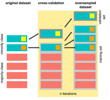
As you see above, SMOTE occurs “during” cross validation and not “prior” to the cross validation process. Synthetic data are created only for the training set without affecting the validation set.
References:
- DEALING WITH IMBALANCED DATA: UNDERSAMPLING, OVERSAMPLING AND PROPER CROSS-VALIDATION
- SMOTE explained for noobs
- Machine Learning - Over-& Undersampling - Python/ Scikit/ Scikit-Imblearn
Near-miss for undersampling algorithm
Near-miss is an algorithm that can help in balancing an imbalanced dataset. It can be grouped under undersampling algorithms and is an efficient way to balance the data. The algorithm does this by looking at the class distribution and randomly eliminating samples from the larger class. When two points belonging to different classes are very close to each other in the distribution, this algorithm eliminates the datapoint of the larger class thereby trying to balance the distribution.
The steps taken by this algorithm are:
The algorithm first calculates the distance between all the points in the larger class and the points in the smaller class. This can make the process of undersampling easier.
Select instances of the larger class that have the shortest distance with the smaller class. These n classes need to be stored for elimination.
If there are m instances of the smaller class then the algorithm will return m*n instances of the larger class.
import imblearn;
imblearn.show_versions(github=True)
System, Dependency Information

**System Information**

* python    : `3.9.13 (main, Aug 25 2022, 18:29:29)  [Clang 12.0.0 ]`
* executable: `/Users/haesongchoi/opt/anaconda3/bin/python`
* machine   : `macOS-10.16-x86_64-i386-64bit`

**Python Dependencies**

* imbalanced-learn: `0.10.1`
* pip       : `22.2.2`
* setuptools: `63.4.1`
* numpy     : `1.21.5`
* scipy     : `1.9.1`
* scikit-learn: `1.2.2`
* Cython    : `0.29.32`
* pandas    : `1.4.4`
* keras     : `None`
* tensorflow: `None`
* joblib    : `1.2.0`
# We will undersample during cross validating
undersample_X = df.drop('Class', axis=1)
undersample_y = df['Class']


for train_index, test_index in sss.split(undersample_X, undersample_y):
    print("Train:", train_index, "Test:", test_index)
    undersample_Xtrain, undersample_Xtest = undersample_X.iloc[train_index], undersample_X.iloc[test_index]
    undersample_ytrain, undersample_ytest = undersample_y.iloc[train_index], undersample_y.iloc[test_index]

undersample_Xtrain = undersample_Xtrain.values
undersample_Xtest = undersample_Xtest.values
undersample_ytrain = undersample_ytrain.values
undersample_ytest = undersample_ytest.values

undersample_accuracy = []
undersample_precision = []
undersample_recall = []
undersample_f1 = []
undersample_auc = []

# Implementing NearMiss Technique
# Distribution of NearMiss (Just to see how it distributes the labels we won't use these variables)
nr = NearMiss()
X_nearmiss, y_nearmiss = NearMiss().fit_resample(undersample_X.values, undersample_y.values)
print('NearMiss Label Distribution: {}'.format(Counter(y_nearmiss)))

# Cross Validating the right way

for train, test in sss.split(undersample_Xtrain, undersample_ytrain):
    undersample_pipeline = imbalanced_make_pipeline(NearMiss(sampling_strategy='majority'), log_reg) # SMOTE happens during Cross Validation not before..
    undersample_model = undersample_pipeline.fit(undersample_Xtrain[train], undersample_ytrain[train])
    undersample_prediction = undersample_model.predict(undersample_Xtrain[test])

    undersample_accuracy.append(undersample_pipeline.score(original_Xtrain[test], original_ytrain[test]))
    undersample_precision.append(precision_score(original_ytrain[test], undersample_prediction))
    undersample_recall.append(recall_score(original_ytrain[test], undersample_prediction))
    undersample_f1.append(f1_score(original_ytrain[test], undersample_prediction))
    undersample_auc.append(roc_auc_score(original_ytrain[test], undersample_prediction))
Train: [ 56957  56958  56959 ... 284804 284805 284806] Test: [    0     1     2 ... 57872 57997 58548]
Train: [     0      1      2 ... 284804 284805 284806] Test: [ 56957  56958  56959 ... 113921 113922 114471]
Train: [     0      1      2 ... 284804 284805 284806] Test: [113923 113924 113925 ... 173553 174323 174911]
Train: [     0      1      2 ... 284804 284805 284806] Test: [170878 170879 170880 ... 231457 231496 231804]
Train: [     0      1      2 ... 231457 231496 231804] Test: [227836 227837 227838 ... 284804 284805 284806]
NearMiss Label Distribution: Counter({0: 492, 1: 492})
# Let's Plot LogisticRegression Learning Curve
from sklearn.model_selection import ShuffleSplit
from sklearn.model_selection import learning_curve

def plot_learning_curve(estimator1, estimator2, estimator3, estimator4, X, y, ylim=None, cv=None,
                        n_jobs=1, train_sizes=np.linspace(.1, 1.0, 5)):
    f, ((ax1, ax2), (ax3, ax4)) = plt.subplots(2,2, figsize=(20,14), sharey=True)
    if ylim is not None:
        plt.ylim(*ylim)
    # First Estimator
    train_sizes, train_scores, test_scores = learning_curve(
        estimator1, X, y, cv=cv, n_jobs=n_jobs, train_sizes=train_sizes)
    train_scores_mean = np.mean(train_scores, axis=1)
    train_scores_std = np.std(train_scores, axis=1)
    test_scores_mean = np.mean(test_scores, axis=1)
    test_scores_std = np.std(test_scores, axis=1)
    ax1.fill_between(train_sizes, train_scores_mean - train_scores_std,
                     train_scores_mean + train_scores_std, alpha=0.1,
                     color="#ff9124")
    ax1.fill_between(train_sizes, test_scores_mean - test_scores_std,
                     test_scores_mean + test_scores_std, alpha=0.1, color="#2492ff")
    ax1.plot(train_sizes, train_scores_mean, 'o-', color="#ff9124",
             label="Training score")
    ax1.plot(train_sizes, test_scores_mean, 'o-', color="#2492ff",
             label="Cross-validation score")
    ax1.set_title("Logistic Regression Learning Curve", fontsize=14)
    ax1.set_xlabel('Training size (m)')
    ax1.set_ylabel('Score')
    ax1.grid(True)
    ax1.legend(loc="best")

    # Second Estimator
    train_sizes, train_scores, test_scores = learning_curve(
        estimator2, X, y, cv=cv, n_jobs=n_jobs, train_sizes=train_sizes)
    train_scores_mean = np.mean(train_scores, axis=1)
    train_scores_std = np.std(train_scores, axis=1)
    test_scores_mean = np.mean(test_scores, axis=1)
    test_scores_std = np.std(test_scores, axis=1)
    ax2.fill_between(train_sizes, train_scores_mean - train_scores_std,
                     train_scores_mean + train_scores_std, alpha=0.1,
                     color="#ff9124")
    ax2.fill_between(train_sizes, test_scores_mean - test_scores_std,
                     test_scores_mean + test_scores_std, alpha=0.1, color="#2492ff")
    ax2.plot(train_sizes, train_scores_mean, 'o-', color="#ff9124",
             label="Training score")
    ax2.plot(train_sizes, test_scores_mean, 'o-', color="#2492ff",
             label="Cross-validation score")
    ax2.set_title("Knears Neighbors Learning Curve", fontsize=14)
    ax2.set_xlabel('Training size (m)')
    ax2.set_ylabel('Score')
    ax2.grid(True)
    ax2.legend(loc="best")

    # Third Estimator
    train_sizes, train_scores, test_scores = learning_curve(
        estimator3, X, y, cv=cv, n_jobs=n_jobs, train_sizes=train_sizes)
    train_scores_mean = np.mean(train_scores, axis=1)
    train_scores_std = np.std(train_scores, axis=1)
    test_scores_mean = np.mean(test_scores, axis=1)
    test_scores_std = np.std(test_scores, axis=1)
    ax3.fill_between(train_sizes, train_scores_mean - train_scores_std,
                     train_scores_mean + train_scores_std, alpha=0.1,
                     color="#ff9124")
    ax3.fill_between(train_sizes, test_scores_mean - test_scores_std,
                     test_scores_mean + test_scores_std, alpha=0.1, color="#2492ff")
    ax3.plot(train_sizes, train_scores_mean, 'o-', color="#ff9124",
             label="Training score")
    ax3.plot(train_sizes, test_scores_mean, 'o-', color="#2492ff",
             label="Cross-validation score")
    ax3.set_title("Support Vector Classifier \n Learning Curve", fontsize=14)
    ax3.set_xlabel('Training size (m)')
    ax3.set_ylabel('Score')
    ax3.grid(True)
    ax3.legend(loc="best")

    # Fourth Estimator
    train_sizes, train_scores, test_scores = learning_curve(
        estimator4, X, y, cv=cv, n_jobs=n_jobs, train_sizes=train_sizes)
    train_scores_mean = np.mean(train_scores, axis=1)
    train_scores_std = np.std(train_scores, axis=1)
    test_scores_mean = np.mean(test_scores, axis=1)
    test_scores_std = np.std(test_scores, axis=1)
    ax4.fill_between(train_sizes, train_scores_mean - train_scores_std,
                     train_scores_mean + train_scores_std, alpha=0.1,
                     color="#ff9124")
    ax4.fill_between(train_sizes, test_scores_mean - test_scores_std,
                     test_scores_mean + test_scores_std, alpha=0.1, color="#2492ff")
    ax4.plot(train_sizes, train_scores_mean, 'o-', color="#ff9124",
             label="Training score")
    ax4.plot(train_sizes, test_scores_mean, 'o-', color="#2492ff",
             label="Cross-validation score")
    ax4.set_title("Decision Tree Classifier \n Learning Curve", fontsize=14)
    ax4.set_xlabel('Training size (m)')
    ax4.set_ylabel('Score')
    ax4.grid(True)
    ax4.legend(loc="best")
    return plt
cv = ShuffleSplit(n_splits=100, test_size=0.2, random_state=42)
plot_learning_curve(log_reg, knears_neighbors, svc, tree_clf, X_train, y_train, (0.87, 1.01), cv=cv, n_jobs=4)
<module 'matplotlib.pyplot' from '/Users/haesongchoi/opt/anaconda3/lib/python3.9/site-packages/matplotlib/pyplot.py'>

from sklearn.metrics import roc_curve
from sklearn.model_selection import cross_val_predict
# Create a DataFrame with all the scores and the classifiers names.

log_reg_pred = cross_val_predict(log_reg, X_train, y_train, cv=5,
                             method="decision_function")

knears_pred = cross_val_predict(knears_neighbors, X_train, y_train, cv=5)

svc_pred = cross_val_predict(svc, X_train, y_train, cv=5,
                             method="decision_function")

tree_pred = cross_val_predict(tree_clf, X_train, y_train, cv=5)
from sklearn.metrics import roc_auc_score

print('Logistic Regression: ', roc_auc_score(y_train, log_reg_pred))
print('KNears Neighbors: ', roc_auc_score(y_train, knears_pred))
print('Support Vector Classifier: ', roc_auc_score(y_train, svc_pred))
print('Decision Tree Classifier: ', roc_auc_score(y_train, tree_pred))
Logistic Regression:  0.9743055555555556
KNears Neighbors:  0.9329545454545455
Support Vector Classifier:  0.9747544893378226
Decision Tree Classifier:  0.9210858585858586
log_fpr, log_tpr, log_thresold = roc_curve(y_train, log_reg_pred)
knear_fpr, knear_tpr, knear_threshold = roc_curve(y_train, knears_pred)
svc_fpr, svc_tpr, svc_threshold = roc_curve(y_train, svc_pred)
tree_fpr, tree_tpr, tree_threshold = roc_curve(y_train, tree_pred)


def graph_roc_curve_multiple(log_fpr, log_tpr, knear_fpr, knear_tpr, svc_fpr, svc_tpr, tree_fpr, tree_tpr):
    plt.figure(figsize=(16,8))
    plt.title('ROC Curve \n Top 4 Classifiers', fontsize=18)
    plt.plot(log_fpr, log_tpr, label='Logistic Regression Classifier Score: {:.4f}'.format(roc_auc_score(y_train, log_reg_pred)))
    plt.plot(knear_fpr, knear_tpr, label='KNears Neighbors Classifier Score: {:.4f}'.format(roc_auc_score(y_train, knears_pred)))
    plt.plot(svc_fpr, svc_tpr, label='Support Vector Classifier Score: {:.4f}'.format(roc_auc_score(y_train, svc_pred)))
    plt.plot(tree_fpr, tree_tpr, label='Decision Tree Classifier Score: {:.4f}'.format(roc_auc_score(y_train, tree_pred)))
    plt.plot([0, 1], [0, 1], 'k--')
    plt.axis([-0.01, 1, 0, 1])
    plt.xlabel('False Positive Rate', fontsize=16)
    plt.ylabel('True Positive Rate', fontsize=16)
    plt.annotate('Minimum ROC Score of 50% \n (This is the minimum score to get)', xy=(0.5, 0.5), xytext=(0.6, 0.3),
                arrowprops=dict(facecolor='#6E726D', shrink=0.05),
                )
    plt.legend()

graph_roc_curve_multiple(log_fpr, log_tpr, knear_fpr, knear_tpr, svc_fpr, svc_tpr, tree_fpr, tree_tpr)
plt.show()

def logistic_roc_curve(log_fpr, log_tpr):
    plt.figure(figsize=(12,8))
    plt.title('Logistic Regression ROC Curve', fontsize=16)
    plt.plot(log_fpr, log_tpr, 'b-', linewidth=2)
    plt.plot([0, 1], [0, 1], 'r--')
    plt.xlabel('False Positive Rate', fontsize=16)
    plt.ylabel('True Positive Rate', fontsize=16)
    plt.axis([-0.01,1,0,1])


logistic_roc_curve(log_fpr, log_tpr)
plt.show()

from sklearn.metrics import precision_recall_curve

precision, recall, threshold = precision_recall_curve(y_train, log_reg_pred)
from sklearn.metrics import recall_score, precision_score, f1_score, accuracy_score
y_pred = log_reg.predict(X_train)

# Overfitting Case
print('---' * 45)
print('Overfitting: \n')
print('Recall Score: {:.2f}'.format(recall_score(y_train, y_pred)))
print('Precision Score: {:.2f}'.format(precision_score(y_train, y_pred)))
print('F1 Score: {:.2f}'.format(f1_score(y_train, y_pred)))
print('Accuracy Score: {:.2f}'.format(accuracy_score(y_train, y_pred)))
print('---' * 45)

# How it should look like
print('---' * 45)
print('How it should be:\n')
print("Accuracy Score: {:.2f}".format(np.mean(undersample_accuracy)))
print("Precision Score: {:.2f}".format(np.mean(undersample_precision)))
print("Recall Score: {:.2f}".format(np.mean(undersample_recall)))
print("F1 Score: {:.2f}".format(np.mean(undersample_f1)))
print('---' * 45)
---------------------------------------------------------------------------------------------------------------------------------------
Overfitting:

Recall Score: 0.96
Precision Score: 0.71
F1 Score: 0.82
Accuracy Score: 0.79
---------------------------------------------------------------------------------------------------------------------------------------
---------------------------------------------------------------------------------------------------------------------------------------
How it should be:

Accuracy Score: 0.58
Precision Score: 0.00
Recall Score: 0.46
F1 Score: 0.00
---------------------------------------------------------------------------------------------------------------------------------------
undersample_y_score = log_reg.decision_function(original_Xtest)
from sklearn.metrics import average_precision_score

undersample_average_precision = average_precision_score(original_ytest, undersample_y_score)

print('Average precision-recall score: {0:0.2f}'.format(
      undersample_average_precision))
Average precision-recall score: 0.04
from sklearn.metrics import precision_recall_curve
import matplotlib.pyplot as plt

fig = plt.figure(figsize=(12,6))

precision, recall, _ = precision_recall_curve(original_ytest, undersample_y_score)

plt.step(recall, precision, color='#004a93', alpha=0.2,
         where='post')
plt.fill_between(recall, precision, step='post', alpha=0.2,
                 color='#48a6ff')

plt.xlabel('Recall')
plt.ylabel('Precision')
plt.ylim([0.0, 1.05])
plt.xlim([0.0, 1.0])
plt.title('UnderSampling Precision-Recall curve: \n Average Precision-Recall Score ={0:0.2f}'.format(
          undersample_average_precision), fontsize=16)
Text(0.5, 1.0, 'UnderSampling Precision-Recall curve: \n Average Precision-Recall Score =0.04')

SMOTE Technique (Over-Sampling):
SMOTE stands for Synthetic Minority Over-sampling Technique. Unlike Random UnderSampling, SMOTE creates new synthetic points in order to have an equal balance of the classes.
Understanding SMOTE:
- Solving the Class Imbalance: SMOTE creates synthetic points from the minority class in order to reach an equal balance between the minority and majority class.
- Location of the synthetic points: SMOTE picks the distance between the closest neighbors of the minority class, in between these distances it creates synthetic points.
- Final Effect: More information is retained since we didn't have to delete any rows unlike in random undersampling.
- Accuracy || Time Tradeoff: Although it is likely that SMOTE will be more accurate than random under-sampling, it will take more time to train since no rows are eliminated as previously stated. ```python from imblearn.over_sampling import SMOTE from sklearn.model_selection import train_test_split, RandomizedSearchCV print('Length of X (train): {} | Length of y (train): {}'.format(len(original_Xtrain), len(original_ytrain))) print('Length of X (test): {} | Length of y (test): {}'.format(len(original_Xtest), len(original_ytest))) # List to append the score and then find the average accuracy_lst = [] precision_lst = [] recall_lst = [] f1_lst = [] auc_lst = [] # Classifier with optimal parameters # log_reg_sm = grid_log_reg.best_estimator_ log_reg_sm = LogisticRegression() rand_log_reg = RandomizedSearchCV(LogisticRegression(), log_reg_params, n_iter=4) # Implementing SMOTE Technique # Cross Validating the right way # Parameters log_reg_params = {"penalty": ['l1', 'l2'], 'C': [0.001, 0.01, 0.1, 1, 10, 100, 1000]} for train, test in sss.split(original_Xtrain, original_ytrain): pipeline = imbalanced_make_pipeline(SMOTE(sampling_strategy='minority'), rand_log_reg) # SMOTE happens during Cross Validation not before.. model = pipeline.fit(original_Xtrain[train], original_ytrain[train]) best_est = rand_log_reg.best_estimator_ prediction = best_est.predict(original_Xtrain[test]) accuracy_lst.append(pipeline.score(original_Xtrain[test], original_ytrain[test])) precision_lst.append(precision_score(original_ytrain[test], prediction)) recall_lst.append(recall_score(original_ytrain[test], prediction)) f1_lst.append(f1_score(original_ytrain[test], prediction)) auc_lst.append(roc_auc_score(original_ytrain[test], prediction)) print('---' * 45) print('') print("accuracy: {}".format(np.mean(accuracy_lst))) print("precision: {}".format(np.mean(precision_lst))) print("recall: {}".format(np.mean(recall_lst))) print("f1: {}".format(np.mean(f1_lst))) print('---' * 45) ```
Length of X (train): 227846 | Length of y (train): 227846
Length of X (test): 56961 | Length of y (test): 56961
---------------------------------------------------------------------------------------------------------------------------------------

accuracy: 0.9413953036891684
precision: 0.061391726484712514
recall: 0.9137293086660175
f1: 0.11320213297425694
---------------------------------------------------------------------------------------------------------------------------------------
```python labels = ['No Fraud', 'Fraud'] smote_prediction = best_est.predict(original_Xtest) print(classification_report(original_ytest, smote_prediction, target_names=labels)) ```
              precision    recall  f1-score   support

    No Fraud       1.00      0.99      0.99     56863
       Fraud       0.11      0.86      0.20        98

    accuracy                           0.99     56961
   macro avg       0.56      0.92      0.60     56961
weighted avg       1.00      0.99      0.99     56961
```python
y_score = best_est.decision_function(original_Xtest)
```
```python
average_precision = average_precision_score(original_ytest, y_score)
print('Average precision-recall score: {0:0.2f}'.format(
average_precision))
```
Average precision-recall score: 0.75```python fig = plt.figure(figsize=(12,6)) precision, recall, _ = precision_recall_curve(original_ytest, y_score) plt.step(recall, precision, color='r', alpha=0.2, where='post') plt.fill_between(recall, precision, step='post', alpha=0.2, color='#F59B00') plt.xlabel('Recall') plt.ylabel('Precision') plt.ylim([0.0, 1.05]) plt.xlim([0.0, 1.0]) plt.title('OverSampling Precision-Recall curve: \n Average Precision-Recall Score ={0:0.2f}'.format( average_precision), fontsize=16) ```
Text(0.5, 1.0, 'OverSampling Precision-Recall curve: \n Average Precision-Recall Score =0.75')
 ```python
# SMOTE Technique (OverSampling) After splitting and Cross Validating
sm = SMOTE(random_state=42) #'ratio = 'minority', ,
# Xsm_train, ysm_train = sm.fit_sample(X_train, y_train)
# This will be the data were we are going to
Xsm_train, ysm_train =sm.fit_resample(original_Xtrain, original_ytrain)
```
```python
# We Improve the score by 2% points approximately
# Implement GridSearchCV and the other models.
# Logistic Regression
t0 = time.time()
log_reg_sm = grid_log_reg.best_estimator_
log_reg_sm.fit(Xsm_train, ysm_train)
t1 = time.time()
print("Fitting oversample data took :{} sec".format(t1 - t0))
```
```python
# SMOTE Technique (OverSampling) After splitting and Cross Validating
sm = SMOTE(random_state=42) #'ratio = 'minority', ,
# Xsm_train, ysm_train = sm.fit_sample(X_train, y_train)
# This will be the data were we are going to
Xsm_train, ysm_train =sm.fit_resample(original_Xtrain, original_ytrain)
```
```python
# We Improve the score by 2% points approximately
# Implement GridSearchCV and the other models.
# Logistic Regression
t0 = time.time()
log_reg_sm = grid_log_reg.best_estimator_
log_reg_sm.fit(Xsm_train, ysm_train)
t1 = time.time()
print("Fitting oversample data took :{} sec".format(t1 - t0))
```
Fitting oversample data took :1.0590651035308838 sec- - - ## SMOTE Oversampling 적용 후 모델학습/예측/평가 - SMOTE를 적용할 때는 반드시 학습 데이터 세트만 오버 샘플링을 해야 합니다. - 검증 데이터 세트나 테스트 데이터 세프를 오버 샘플링할 경우 결국은 original dataset가 아닌 Dataset에서 검증 또는 테스트를 수행하기 때문에 올바른 검증/테스트가 될 수 없다. ```python from imblearn.over_sampling import SMOTE smote = SMOTE(random_state=0) X_train_over, y_train_over =smote.fit_resample(X_train, y_train) #only train set print('SMOTE 적용 전: ', X_train.shape, y_train.shape) print('SMOTE 적용 전 label값 분포: \n', pd.Series(y_train).value_counts()) #SMOTE 적용 후 label값에서 0과 1의 분포가 동일하게 생성됨. print('SMOTE 적용 후: ', X_train_over.shape, y_train_over.shape) print('SMOTE 적용 후 label값 분포: \n', pd.Series(y_train_over).value_counts()) ```
SMOTE 적용 전:  (756, 30) (756,)
SMOTE 적용 전 label값 분포:
 0    396
1    360
dtype: int64
SMOTE 적용 후:  (792, 30) (792,)
SMOTE 적용 후 label값 분포:
 0    396
1    396
dtype: int64
```python lr_clf = LogisticRegression() get_model_train_eval(lr_clf, ftr_train=X_train_over, ftr_test=X_test, tgt_train=y_train_over, tgt_test=y_test) ```
confusion matrix
[[90  3]
 [ 8 89]]
accuracy: 0.9421, precision: 0.9674, recall(sensitivity): 0.9175, f1_score: 0.9418, AUC: 0.9717
- precision이 급격하게 낮아짐. Oversampling으로 인해 실제 원본 데이터의 유형보다 너무나 많은 Class=1데이터를 학습하면서 실제 테스트 데이터 세으텡서 예측을 지나치게 Class=1으로 적용해 precision이 떨어지게 됨. - 좋은 SMOTE 패키지일수록 recall(sensitivity)은 증가율은 높이고 precision의 감소율은 낮출 수 있도록 효과적으로 데이터를 증식한다. ```python lgbm_clf = LGBMClassifier(n_estimators=1000, num_leaves=64, n_jobs=-1, boost_from_average=False) get_model_train_eval(lgbm_clf, ftr_train=X_train_over, ftr_test=X_test, tgt_train=y_train_over, tgt_test=y_test) # Recall : 82.88% 에서 84.93으로 증가했음. ```
confusion matrix
[[92  1]
 [ 5 92]]
accuracy: 0.9684, precision: 0.9892, recall(sensitivity): 0.9485, f1_score: 0.9684, AUC: 0.9818
# Test Data with Logistic Regression ### Summary:
- Random UnderSampling: We will evaluate the final performance of the classification models in the random undersampling subset. Keep in mind that this is not the data from the original dataframe.
- Classification Models: The models that performed the best were logistic regression and support vector classifier (SVM)
 ```python
from sklearn.metrics import classification_report
print('Logistic Regression:')
print(classification_report(y_test, y_pred_log_reg))
print('KNears Neighbors:')
print(classification_report(y_test, y_pred_knear))
print('Support Vector Classifier:')
print(classification_report(y_test, y_pred_svc))
print('Support Vector Classifier:')
print(classification_report(y_test, y_pred_tree))
```
```python
from sklearn.metrics import classification_report
print('Logistic Regression:')
print(classification_report(y_test, y_pred_log_reg))
print('KNears Neighbors:')
print(classification_report(y_test, y_pred_knear))
print('Support Vector Classifier:')
print(classification_report(y_test, y_pred_svc))
print('Support Vector Classifier:')
print(classification_report(y_test, y_pred_tree))
```
Logistic Regression:
              precision    recall  f1-score   support

           0       0.93      0.99      0.96        93
           1       0.99      0.93      0.96        97

    accuracy                           0.96       190
   macro avg       0.96      0.96      0.96       190
weighted avg       0.96      0.96      0.96       190

KNears Neighbors:
              precision    recall  f1-score   support

           0       0.92      0.98      0.95        93
           1       0.98      0.92      0.95        97

    accuracy                           0.95       190
   macro avg       0.95      0.95      0.95       190
weighted avg       0.95      0.95      0.95       190

Support Vector Classifier:
              precision    recall  f1-score   support

           0       0.92      0.97      0.94        93
           1       0.97      0.92      0.94        97

    accuracy                           0.94       190
   macro avg       0.94      0.94      0.94       190
weighted avg       0.94      0.94      0.94       190

Support Vector Classifier:
              precision    recall  f1-score   support

           0       0.90      0.98      0.94        93
           1       0.98      0.90      0.94        97

    accuracy                           0.94       190
   macro avg       0.94      0.94      0.94       190
weighted avg       0.94      0.94      0.94       190
```python
# Final Score in the test set of logistic regression
from sklearn.metrics import accuracy_score
# Logistic Regression with Under-Sampling
y_pred = log_reg.predict(X_test)
undersample_score = accuracy_score(y_test, y_pred)
# Logistic Regression with SMOTE Technique (Better accuracy with SMOTE t)
y_pred_sm = best_est.predict(original_Xtest)
oversample_score = accuracy_score(original_ytest, y_pred_sm)
d = {'Technique': ['Random UnderSampling', 'Oversampling (SMOTE)'], 'Score': [undersample_score, oversample_score]}
final_df = pd.DataFrame(data=d)
# Move column
score = final_df['Score']
final_df.drop('Score', axis=1, inplace=True)
final_df.insert(1, 'Score', score)
# Note how high is accuracy score it can be misleading!
final_df
```
| Technique | Score | |
|---|---|---|
| 0 | Random UnderSampling | 0.957895 |
| 1 | Oversampling (SMOTE) | 0.988027 |
**Note:** One last thing, predictions and accuracies may be subjected to change since I implemented data shuffling on both types of dataframes. The main thing is to see if our models are able to correctly classify no fraud and fraud transactions. I will bring more updates, stay tuned!
Leave a comment