Kaggle-House Prices - Advanced Regression Techniques

House price regression Techniques

• Goal: We predict the final price of each home based on the given features.

• Metric: Root-Mean-Squared-Error (RMSE) between the logarithm of the predicted value and the logarithm of the observed sales price.

• Data

  • 79 features describing (almost) every aspect of residential homes in Ames, Iowa, y=salePrice

  • Feature description

import pandas as pd
import numpy as np
import seaborn as sns
import matplotlib.pyplot as plt
%matplotlib inline

from sklearn.linear_model import LinearRegression, Ridge, Lasso
from sklearn.model_selection import train_test_split
from sklearn.metrics import mean_squared_error

import warnings
warnings.filterwarnings('ignore')

Dataset

house_df_org = pd.read_csv('input/house_price.csv')
house_df = house_df_org.copy()
df.head(3)

	Id	MSSubClass	MSZoning	LotFrontage	LotArea	Street	Alley	LotShape	LandContour	Utilities	...	PoolArea	PoolQC	Fence	MiscFeature	MiscVal	MoSold	YrSold	SaleType	SaleCondition	SalePrice
0	1	60	RL	65.0	8450	Pave	NaN	Reg	Lvl	AllPub	...	0	NaN	NaN	NaN	0	2	2008	WD	Normal	208500
1	2	20	RL	80.0	9600	Pave	NaN	Reg	Lvl	AllPub	...	0	NaN	NaN	NaN	0	5	2007	WD	Normal	181500
2	3	60	RL	68.0	11250	Pave	NaN	IR1	Lvl	AllPub	...	0	NaN	NaN	NaN	0	9	2008	WD	Normal	223500

3 rows × 81 columns

house_df.shape

(1460, 81)

#df.info()
house_df.describe()

	Id	MSSubClass	LotFrontage	LotArea	OverallQual	OverallCond	YearBuilt	YearRemodAdd	MasVnrArea	BsmtFinSF1	...	WoodDeckSF	OpenPorchSF	EnclosedPorch	3SsnPorch	ScreenPorch	PoolArea	MiscVal	MoSold	YrSold	SalePrice
count	1460.000000	1460.000000	1201.000000	1460.000000	1460.000000	1460.000000	1460.000000	1460.000000	1452.000000	1460.000000	...	1460.000000	1460.000000	1460.000000	1460.000000	1460.000000	1460.000000	1460.000000	1460.000000	1460.000000	1460.000000
mean	730.500000	56.897260	70.049958	10516.828082	6.099315	5.575342	1971.267808	1984.865753	103.685262	443.639726	...	94.244521	46.660274	21.954110	3.409589	15.060959	2.758904	43.489041	6.321918	2007.815753	180921.195890
std	421.610009	42.300571	24.284752	9981.264932	1.382997	1.112799	30.202904	20.645407	181.066207	456.098091	...	125.338794	66.256028	61.119149	29.317331	55.757415	40.177307	496.123024	2.703626	1.328095	79442.502883
min	1.000000	20.000000	21.000000	1300.000000	1.000000	1.000000	1872.000000	1950.000000	0.000000	0.000000	...	0.000000	0.000000	0.000000	0.000000	0.000000	0.000000	0.000000	1.000000	2006.000000	34900.000000
25%	365.750000	20.000000	59.000000	7553.500000	5.000000	5.000000	1954.000000	1967.000000	0.000000	0.000000	...	0.000000	0.000000	0.000000	0.000000	0.000000	0.000000	0.000000	5.000000	2007.000000	129975.000000
50%	730.500000	50.000000	69.000000	9478.500000	6.000000	5.000000	1973.000000	1994.000000	0.000000	383.500000	...	0.000000	25.000000	0.000000	0.000000	0.000000	0.000000	0.000000	6.000000	2008.000000	163000.000000
75%	1095.250000	70.000000	80.000000	11601.500000	7.000000	6.000000	2000.000000	2004.000000	166.000000	712.250000	...	168.000000	68.000000	0.000000	0.000000	0.000000	0.000000	0.000000	8.000000	2009.000000	214000.000000
max	1460.000000	190.000000	313.000000	215245.000000	10.000000	9.000000	2010.000000	2010.000000	1600.000000	5644.000000	...	857.000000	547.000000	552.000000	508.000000	480.000000	738.000000	15500.000000	12.000000	2010.000000	755000.000000

8 rows × 38 columns

Null data check

house_df.isnull().sum()[house_df.isnull().sum()>0].sort_values(ascending=False)

PoolQC          1453
MiscFeature     1406
Alley           1369
Fence           1179
FireplaceQu      690
LotFrontage      259
GarageType        81
GarageYrBlt       81
GarageFinish      81
GarageQual        81
GarageCond        81
BsmtExposure      38
BsmtFinType2      38
BsmtFinType1      37
BsmtCond          37
BsmtQual          37
MasVnrArea         8
MasVnrType         8
Electrical         1
dtype: int64

# Drop the features containing many NaNs.
house_df.drop(['PoolQC', 'MiscFeature', 'Alley', 'Fence','FireplaceQu', 'Id'], axis=1, inplace=True)

house_df.fillna(house_df.mean(), inplace=True)

# Features type
house_df.dtypes.value_counts()

object     38
int64      34
float64     3
dtype: int64

The distribution of Target Label

plt.title('Original Sale Price Histogram')
sns.distplot(house_df['SalePrice']) # skewed

<AxesSubplot:title={'center':'Original Sale Price Histogram'}, xlabel='SalePrice', ylabel='Density'>

plt.title('Log transformed Sale Price Histogram')
log_SalePrice =np.log1p(house_df['SalePrice'])
sns.distplot(log_SalePrice)

<AxesSubplot:title={'center':'Log Transformed Sale Price Histogram'}, xlabel='SalePrice', ylabel='Density'>

house_df['log_SalePrice'] = log_SalePrice
house_df.drop(['SalePrice'], axis=1, inplace=True)

nulls = house_df.isnull().sum()[house_df.isnull().sum()>0]
house_df[nulls.index].dtypes

MasVnrType      object
BsmtQual        object
BsmtCond        object
BsmtExposure    object
BsmtFinType1    object
BsmtFinType2    object
Electrical      object
GarageType      object
GarageFinish    object
GarageQual      object
GarageCond      object
dtype: object

Feature Engineering/ Model Learning

One-hot encoding

# One-hot encoding for object features with null values
house_df_ohe = pd.get_dummies(house_df)
print('Before One-hot:', house_df.shape)
print('After One-hot:', house_df_ohe.shape)
print(house_df_ohe.isnull().sum()[house_df_ohe.isnull().sum()>0]) 

Before One-hot: (1460, 75)
After One-hot: (1460, 271)
Series([], dtype: int64)

Split the training set and test set

y_target = house_df_ohe['log_SalePrice']
X_features = house_df_ohe.drop('log_SalePrice', axis=1, inplace=False)
X_train, X_test, y_train, y_test = train_test_split(X_features, y_target, test_size=0.2, random_state=156)

Linear Regression Model Learning/Prediction/Evaluation

def get_rmse(model):
    model.fit(X_train, y_train)
    pred = model.predict(X_test)
    rmse = np.sqrt(mean_squared_error(y_test, pred)) #Because y is already logged.
    print('RMSE of',model.__class__.__name__, np.round(rmse,3))
    return rmse

def get_rmses(models):
    rmses=[]
    for model in models:
        rmse = get_rmse(model)
        rmses.append(rmse)

lr_reg = LinearRegression()
lr_reg.fit(X_train, y_train)

ridge_reg = Ridge()
ridge_reg.fit(X_train, y_train)

lasso_reg = Lasso()
lasso_reg.fit(X_train, y_train)

models = [lr_reg, ridge_reg, lasso_reg]
get_rmses(models)

RMSE of LinearRegression 0.132
RMSE of Ridge 0.128
RMSE of Lasso 0.176

Coefficient Visualization

def get_top_bottom_coef(model):
    coef = pd.Series(model.coef_, index=X_features.columns)
    coef_high = coef.sort_values(ascending=False).head(10)
    coef_low = coef.sort_values(ascending=False).tail(10)
    return coef_high, coef_low

def visualize_coefficient(models):

    fig, axs = plt.subplots(figsize=(24,10),nrows=1, ncols=3)
    fig.tight_layout() 
    
    for i_num, model in enumerate(models):

        coef_high, coef_low = get_top_bottom_coef(model) # The top 10 and the bottom 10 coefficients.
        coef_concat = pd.concat( [coef_high , coef_low] )
        axs[i_num].set_title(model.__class__.__name__+' Coeffiecents', size=25)
        axs[i_num].tick_params(axis="y",direction="in", pad=-120)
        for label in (axs[i_num].get_xticklabels() + axs[i_num].get_yticklabels()):
            label.set_fontsize(22)
        sns.barplot(x=coef_concat.values, y=coef_concat.index , ax=axs[i_num])

#lr_reg, ridge_reg, lasso_reg Model  

models = [lr_reg, ridge_reg, lasso_reg]
visualize_coefficient(models)

Cross Validation

from sklearn.model_selection import cross_val_score

def get_avg_rmse_cv(models):
    for model in models:
        rmse_list = np.sqrt(-cross_val_score(model, X_features, y_target,
                                             scoring="neg_mean_squared_error", cv = 5))
        rmse_avg = np.mean(rmse_list)
        print('\n{0} The list of RMSEs: {1}'.format( model.__class__.__name__, np.round(rmse_list, 3)))
        print('{0} mean RMSE: {1}'.format( model.__class__.__name__, np.round(rmse_avg, 3)))

models = [lr_reg, ridge_reg, lasso_reg]
get_avg_rmse_cv(models)

LinearRegression The list of RMSEs: [0.135 0.165 0.168 0.111 0.198]
LinearRegression mean RMSE: 0.155

Ridge The list of RMSEs: [0.115 0.148 0.13  0.118 0.186]
Ridge mean RMSE: 0.139

Lasso The list of RMSEs: [0.11  0.15  0.125 0.114 0.193]
Lasso mean RMSE: 0.139

Hyperparameter tuning

from sklearn.model_selection import GridSearchCV

def print_best_params(model, params):
    grid_model = GridSearchCV(model, param_grid=params, 
                              scoring='neg_mean_squared_error', cv=5)
    grid_model.fit(X_features, y_target)
    rmse = np.sqrt(-1* grid_model.best_score_)
    print('{0} RMSE on the best parameters: {1}, The best alpha:{2}'.format(model.__class__.__name__,
                                        np.round(rmse, 4), grid_model.best_params_))
    return grid_model.best_estimator_

ridge_params = { 'alpha':[0.05, 0.1, 1, 5, 8, 10, 12, 15, 20] }
lasso_params = { 'alpha':[0.001, 0.005, 0.008, 0.05, 0.03, 0.1, 0.5, 1,5, 10] }
best_rige = print_best_params(ridge_reg, ridge_params)
best_lasso = print_best_params(lasso_reg, lasso_params)

Ridge RMSE on the best parameters: 0.1418, The best alpha:{'alpha': 12}
Lasso RMSE on the best parameters: 0.142, The best alpha:{'alpha': 0.001}

lr_reg = LinearRegression()
lr_reg.fit(X_train, y_train)
ridge_reg = Ridge(alpha=12)
ridge_reg.fit(X_train, y_train)
lasso_reg = Lasso(alpha=0.001)
lasso_reg.fit(X_train, y_train)

models = [lr_reg, ridge_reg, lasso_reg]
get_rmses(models)

models = [lr_reg, ridge_reg, lasso_reg]
visualize_coefficient(models)

RMSE of LinearRegression 0.132
RMSE of Ridge 0.124
RMSE of Lasso 0.12

Transform very skewed dataset

from scipy.stats import skew

# Select int/float, not object.
features_index = house_df.dtypes[house_df.dtypes != 'object'].index
skew_features = house_df[features_index].apply(lambda x : skew(x))

# Skew > 1 
skew_features_top = skew_features[skew_features > 1]
print(skew_features_top.sort_values(ascending=False))

PoolArea         14.348342
3SsnPorch         7.727026
LowQualFinSF      7.452650
MiscVal           5.165390
BsmtHalfBath      3.929022
KitchenAbvGr      3.865437
ScreenPorch       3.147171
BsmtFinSF2        2.521100
EnclosedPorch     2.110104
dtype: float64

house_df[skew_features_top.index] = np.log1p(house_df[skew_features_top.index])

house_df_ohe = pd.get_dummies(house_df)
y_target = house_df_ohe['log_SalePrice']
X_features = house_df_ohe.drop('log_SalePrice',axis=1, inplace=False)
X_train, X_test, y_train, y_test = train_test_split(X_features, y_target, test_size=0.2, random_state=156)


ridge_params = { 'alpha':[0.05, 0.1, 1, 5, 8, 10, 12, 15, 20] }
lasso_params = { 'alpha':[0.001, 0.005, 0.008, 0.05, 0.03, 0.1, 0.5, 1,5, 10] }
best_ridge = print_best_params(ridge_reg, ridge_params)
best_lasso = print_best_params(lasso_reg, lasso_params)

Ridge RMSE on the best parameters: 0.1276, The best alpha:{'alpha': 10}
Lasso RMSE on the best parameters: 0.1251, The best alpha:{'alpha': 0.001}

lr_reg = LinearRegression()
lr_reg.fit(X_train, y_train)
ridge_reg = Ridge(alpha=10)
ridge_reg.fit(X_train, y_train)
lasso_reg = Lasso(alpha=0.001)
lasso_reg.fit(X_train, y_train)


models = [lr_reg, ridge_reg, lasso_reg]
get_rmses(models)

models = [lr_reg, ridge_reg, lasso_reg]
visualize_coefficient(models)

RMSE of LinearRegression 0.129
RMSE of Ridge 0.121
RMSE of Lasso 0.117

Outlier Removal

plt.scatter(x = house_df_org['GrLivArea'], y = house_df_org['SalePrice'])
plt.ylabel('SalePrice', fontsize=15)
plt.xlabel('GrLivArea', fontsize=15)
plt.show()

cond1 = house_df_ohe['GrLivArea'] > np.log1p(4000) #Since they have been logged, the condition has to be logged.
cond2 = house_df_ohe['log_SalePrice'] < np.log1p(500000)
outlier_index = house_df_ohe[cond1 & cond2].index

print('Outlier index :', outlier_index.values)
print('house_df_ohe shape before outlier removal:', house_df_ohe.shape)

# Delet outliers.
house_df_ohe.drop(outlier_index , axis=0, inplace=True)
print('house_df_ohe shape after outlier removal:', house_df_ohe.shape)

Outlier index : [ 523 1298]
house_df_ohe shape before outlier removal: (1460, 271)
house_df_ohe shape after outlier removal: (1458, 271)

y_target = house_df_ohe['log_SalePrice']
X_features = house_df_ohe.drop('log_SalePrice',axis=1, inplace=False)
X_train, X_test, y_train, y_test = train_test_split(X_features, y_target, test_size=0.2, random_state=156)

ridge_params = { 'alpha':[0.05, 0.1, 1, 5, 8, 10, 12, 15, 20] }
lasso_params = { 'alpha':[0.001, 0.005, 0.008, 0.05, 0.03, 0.1, 0.5, 1,5, 10] }
best_ridge = print_best_params(ridge_reg, ridge_params)
best_lasso = print_best_params(lasso_reg, lasso_params)

Ridge RMSE on the best parameters: 0.1125, The best alpha:{'alpha': 8}
Lasso RMSE on the best parameters: 0.1122, The best alpha:{'alpha': 0.001}

lr_reg = LinearRegression()
lr_reg.fit(X_train, y_train)
ridge_reg = Ridge(alpha=8)
ridge_reg.fit(X_train, y_train)
lasso_reg = Lasso(alpha=0.001)
lasso_reg.fit(X_train, y_train)

# RMSE on each model
models = [lr_reg, ridge_reg, lasso_reg]
get_rmses(models)

# Visualization of important coefficients
models = [lr_reg, ridge_reg, lasso_reg]
visualize_coefficient(models)

RMSE of LinearRegression 0.129
RMSE of Ridge 0.103
RMSE of Lasso 0.1

Tree-based Regression Learning/Prediction/Evaluation

from xgboost import XGBRegressor

xgb_params = {'n_estimators':[1000]}
xgb_reg = XGBRegressor(n_estimators=1000, learning_rate=0.05, 
                       colsample_bytree=0.5, subsample=0.8)
best_xgb = print_best_params(xgb_reg, xgb_params)

XGBRegressor RMSE on the best parameters: 0.1198, The best alpha:{'n_estimators': 1000}

from lightgbm import LGBMRegressor

lgbm_params = {'n_estimators':[1000]}
lgbm_reg = LGBMRegressor(n_estimators=1000, learning_rate=0.05, num_leaves=4, 
                         subsample=0.6, colsample_bytree=0.4, reg_lambda=10, n_jobs=-1)
best_lgbm = print_best_params(lgbm_reg, lgbm_params)

LGBMRegressor RMSE on the best parameters: 0.1163, The best alpha:{'n_estimators': 1000}

def get_top_features(model):
    ftr_importances_values = model.feature_importances_
    ftr_importances = pd.Series(ftr_importances_values, index=X_features.columns  )
    ftr_top20 = ftr_importances.sort_values(ascending=False)[:20]
    return ftr_top20

def visualize_ftr_importances(models):
    fig, axs = plt.subplots(figsize=(24,10),nrows=1, ncols=2)
    fig.tight_layout() 
    for i_num, model in enumerate(models):
        ftr_top20 = get_top_features(model)
        axs[i_num].set_title(model.__class__.__name__+' Feature Importances', size=25)

        for label in (axs[i_num].get_xticklabels() + axs[i_num].get_yticklabels()):
            label.set_fontsize(22)
        sns.barplot(x=ftr_top20.values, y=ftr_top20.index , ax=axs[i_num])


models = [best_xgb, best_lgbm]
visualize_ftr_importances(models)

Stacking

Weighted Averaging

def get_rmse_pred(preds):
    for key in preds.keys():
        pred_value = preds[key]
        mse = mean_squared_error(y_test , pred_value)
        rmse = np.sqrt(mse)
        print('RMSE of {0}: {1}'.format(key, rmse))

# Training each model
ridge_reg = Ridge(alpha=8)
ridge_reg.fit(X_train, y_train)
lasso_reg = Lasso(alpha=0.001)
lasso_reg.fit(X_train, y_train)

# Prediction
ridge_pred = ridge_reg.predict(X_test)
lasso_pred = lasso_reg.predict(X_test)

# Weighted average of models
pred = 0.4 * ridge_pred + 0.6 * lasso_pred
preds = {'Mixed': pred,
         'Ridge': ridge_pred,
         'Lasso': lasso_pred}

#Final mixed model based on ridge and lasso
get_rmse_pred(preds)

RMSE of Mixed: 0.09970842737250571
RMSE of Ridge: 0.10313299412082655
RMSE of Lasso: 0.09991843167945542

xgb_reg = XGBRegressor(n_estimators=1000, learning_rate=0.05, 
                       colsample_bytree=0.5, subsample=0.8)
lgbm_reg = LGBMRegressor(n_estimators=1000, learning_rate=0.05, num_leaves=4, 
                         subsample=0.6, colsample_bytree=0.4, reg_lambda=10, n_jobs=-1)
xgb_reg.fit(X_train, y_train)
lgbm_reg.fit(X_train, y_train)
xgb_pred = xgb_reg.predict(X_test)
lgbm_pred = lgbm_reg.predict(X_test)

pred = 0.5 * xgb_pred + 0.5 * lgbm_pred
preds = {'Mixed': pred,
         'XGBM': xgb_pred,
         'LGBM': lgbm_pred}
        
get_rmse_pred(preds)

RMSE of Mixed: 0.10277689340617208
RMSE of XGBM: 0.10946473825650248
RMSE of LGBM: 0.10382510019327311

Meta-classifier

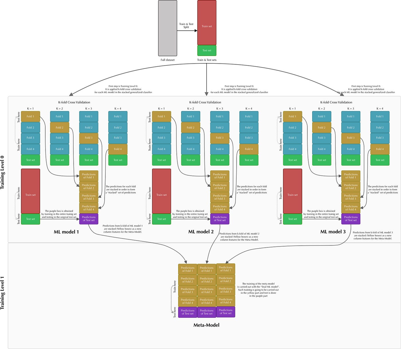
from sklearn.model_selection import KFold
from sklearn.metrics import mean_absolute_error


def get_stacking_base_datasets(model, X_train_n, y_train_n, X_test_n, n_folds ):

    kf = KFold(n_splits=n_folds, shuffle=True, random_state=0)

    train_fold_pred = np.zeros((X_train_n.shape[0] ,1 ))
    test_pred = np.zeros((X_test_n.shape[0],n_folds))
    print(model.__class__.__name__ , ' Start model')
    
    for folder_counter , (train_index, valid_index) in enumerate(kf.split(X_train_n)):

        print('\t fold-set: ',folder_counter,' Start ')
        X_tr = X_train_n[train_index] 
        y_tr = y_train_n[train_index] 
        X_te = X_train_n[valid_index]  
        
 
        model.fit(X_tr , y_tr)       
   
        train_fold_pred[valid_index, :] = model.predict(X_te).reshape(-1,1)

        test_pred[:, folder_counter] = model.predict(X_test_n)
            

    test_pred_mean = np.mean(test_pred, axis=1).reshape(-1,1)    
    
    
    return train_fold_pred , test_pred_mean

# get_stacking_base_datasets( ) uses numpy ndarray.
X_train_n = X_train.values
X_test_n = X_test.values
y_train_n = y_train.values

# Training/ test data based on each base model.
ridge_train, ridge_test = get_stacking_base_datasets(ridge_reg, X_train_n, y_train_n, X_test_n, 5)
lasso_train, lasso_test = get_stacking_base_datasets(lasso_reg, X_train_n, y_train_n, X_test_n, 5)
xgb_train, xgb_test = get_stacking_base_datasets(xgb_reg, X_train_n, y_train_n, X_test_n, 5)  
lgbm_train, lgbm_test = get_stacking_base_datasets(lgbm_reg, X_train_n, y_train_n, X_test_n, 5)

Ridge  Start model
	 fold-set:  0  Start 
	 fold-set:  1  Start 
	 fold-set:  2  Start 
	 fold-set:  3  Start 
	 fold-set:  4  Start 
Lasso  Start model
	 fold-set:  0  Start 
	 fold-set:  1  Start 
	 fold-set:  2  Start 
	 fold-set:  3  Start 
	 fold-set:  4  Start 
XGBRegressor  Start model
	 fold-set:  0  Start 
	 fold-set:  1  Start 
	 fold-set:  2  Start 
	 fold-set:  3  Start 
	 fold-set:  4  Start 
LGBMRegressor  Start model
	 fold-set:  0  Start 
	 fold-set:  1  Start 
	 fold-set:  2  Start 
	 fold-set:  3  Start 
	 fold-set:  4  Start 

# Stacking training/ test data based on each base model
Stack_final_X_train = np.concatenate((ridge_train, lasso_train, 
                                      xgb_train, lgbm_train), axis=1)
Stack_final_X_test = np.concatenate((ridge_test, lasso_test, 
                                     xgb_test, lgbm_test), axis=1)

# Final meta model = Lasso model. 
meta_model_lasso = Lasso(alpha=0.0005)

# Evaluation of RMSE 
meta_model_lasso.fit(Stack_final_X_train, y_train)
final = meta_model_lasso.predict(Stack_final_X_test)
mse = mean_squared_error(y_test , final)
rmse = np.sqrt(mse)
print('RMSE of stacking regression model:', rmse)

RMSE of stacking regression model: 0.09827602546454259