Sorting Algorithm

Selection Sort

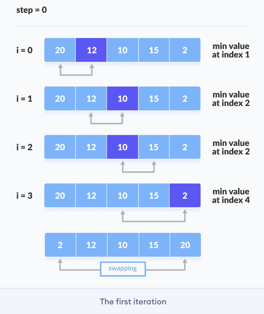
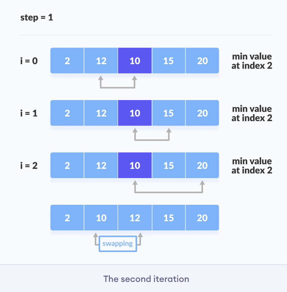
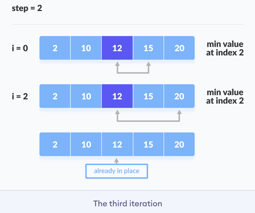
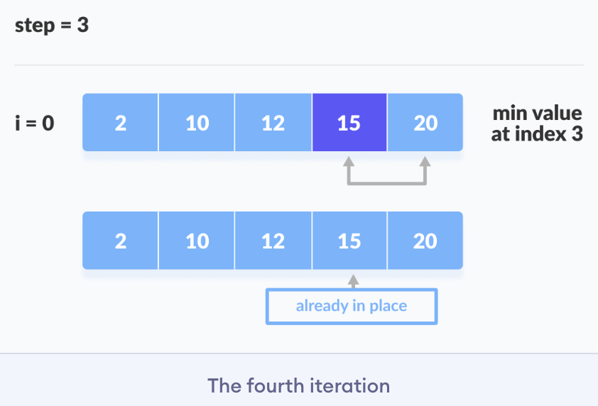
Selection sort is a sorting algorithm that selects the smallest element from an unsorted list in each iteration and places that element at the beginning of the u nsorted list.

Working of Selection Sort

1. Set the first element as a minimum.
2. After each iteration, a minimum is placed in the front of the unsorted list.
3. Swap the first with minimum.
4. For each iteration, indexing starts from the first unsorted element. Steps 1 to 3 are repeated until all the elements are placed in their correct positions.

Source code

array  [7,5,9,0,3,1,6,2,4,8]

for i in range(len(array)):
	min_index = i  # 가장 작은 원소의 인덱스
    for j in range(i+1, len(array)):
    	if array[min_index]>array[j]:
        	min_index = j
    array[i], array[min_index] = array[min_index], array[i]  # swap
print(array)

#[실행 결과]
[0,1,2,3,4,5,6,7,8,9]

Time complexity

• 선택 정렬은 N번 만큼 가장 작은 수를 찾아서 맨 앞으로 보내야 한다.
• 구현 방식에 따라서 사소한 오차는 있을 수 있지만, 전체 연산 횟수는 $N + (N-1) + (N-2) + … + 2 = (N^2 + N + 2)/2 = O(N^2)$.

Insertion Sort

Insertion sort is a sorting algorithm that places an unsorted element at its suitable place in each iteration.

• Insertion sort works similarly as we sort cards in our hands in a card game.
• 처리되지 않은 데이터를 하나씩 골라 적절한 위치에 삽입한다.
• 선택 정렬에 비해 구현 난이도가 높은 편이지만, 일반적으로 더 효율적으로 동작한다.

Working on Sorting Sort

• The first element in the array is assumed to be sorted. Take the second element and store it separately in key.
• Compare key with the first element. If the first element is greater than key, then key is placed in front of the first element.
• Now, the first two elements are sorted. Take the third element and compare it with the elements on the left of it. Placed it just behind the element smaller than it. If no element is smaller than it, place it at the beginning of the array.
• Similarly, place every unsorted element in its correct position.

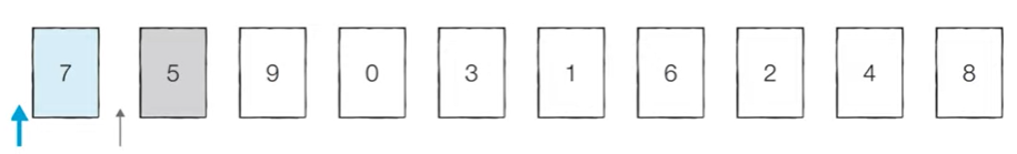
[Step 0] 첫 번째 데이터 ‘7’은 그 자체로 정렬이 되어 있다고 판단하고, 두 번째 데이터인 ‘5’가 어떤 위치로 들어갈지 판단한다. ‘7’의 왼쪽으로 들어가거나 오른쪽으로 들어가거나 두 경우만 존재한다.

[Step 1] 이어서 ‘9’가 어떤 위치로 들어갈지 판단한다.

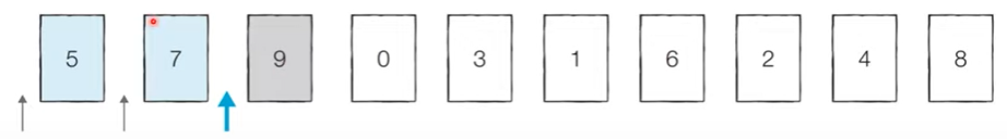
• ‘9’는 차례대로 왼쪽에 있는 데이터와 비교해서 왼쪽 데이터보다 더 작다면 위치를 바꿔 주고 그렇지 않다면 그냥 그자리에 머물러 있도록 한다.
• ‘9’는 ‘7’보다 더 크기 때문에 현재 위치 그대로 내버려둔다.

[Step 2] 이어서 ‘0’이 어떤 위치로 들어갈지 판단한다.

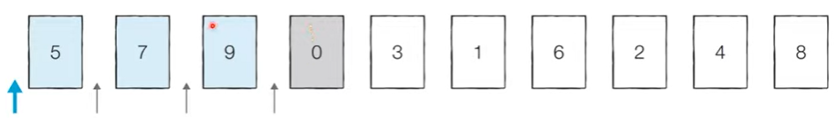
• ‘0’은 ‘9’,’7’,’5’와 비교했을 때 모두 작기 때문에 ‘5’의 왼쪽에 위치한다.

Source code

array = [7,5,9,0,3,1,6,2,4,8]

for i in range(1, len(array)):  # 2번째 원소부터 시작, 인덱스 i부터 1까지 1씩 감소하며 반복하는 문법
	for j in range(i, 0, -1):  #삽입하고자 하는 원소의 위치. 한 칸씩 왼쪽으로 이동
    	if array[j] < array[j-1]:
        	array[j], array[j-1] = array[j-1], array[j] #swap
        else:  # 자기보다 작은 데이터를 만나면 그 위치에서 멈춤
        	break

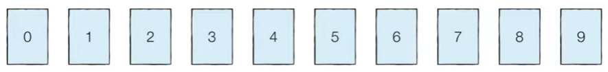
print(array) #[0,1,2,3,4,5,6,7,8,9]

Time Complexity

• 삽입 정렬의 시간 복잡도는 $O(N^2)$이며, 선택 정렬과 마찬가지로 반복문이 두 번 중첩되어 사용된다.
• 삽입 정렬은 현재 리스트의 데이터가 거의 정렬되어 있는 상태라면 매우 빠르게 동작한다. 최선의 경우 O(N)의 시간 복잡도를 가진다.

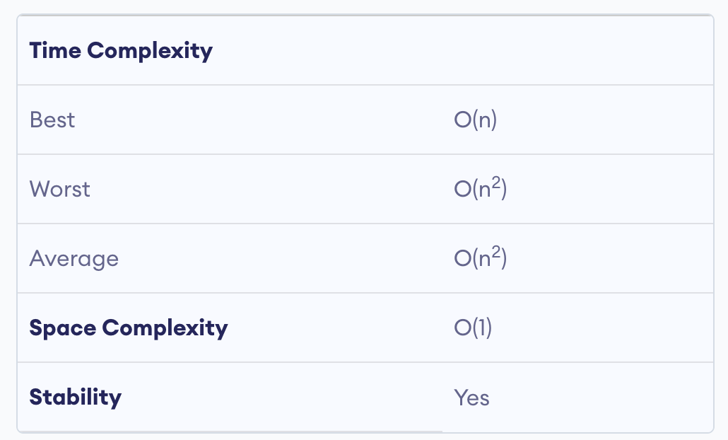
Time Complexities

• Worst Case Complexity: $O(n^2)$ Suppose, an array is in ascending order, and you want to sort it in descending order. In this case, worst-case complexity occurs.

  Each element has to be compared with each of the other elements, so, for every nth element, (n-1) number of comparisons are made.

  Thus, the total number of comparisons = $n*(n-1) \sim n^2$

• Best Case Complexity: $O(n)$ When the array is already sorted, the outer loop runs for n number of times, whereas the inner loop does not run at all. So, there is only n number of comparisons. Thus, complexity is linear.

• Average Case Complexity: $O(n^2)$ It occurs when the elements of an array are in jumbled order (neither ascending nor descending).

Space Complexity

Space complexity is O(1) because an extra variable key is used.

Merge sort

• Merge Sort is one of the most popular sorting algorithms that is based on the principle of Divide and Conquer Algorithm.
• A problem is divided into multiple sub-problems. Each sub-problem is solved individually (Using the Divide and Conquer technique, we divide a problem into subproblems.).
• Finally, sub-problems are combined to form the final solution.

Suppose we had to sort an array A. A subproblem would be to sort a sub-section of this array starting at index p and ending at index r, denoted as A[p..r].

Divide

If q is the halfway point between p and r, then we can split the subarray A[p..r] into two arrays A[p..q] and A[q+1, r].

Conquer

In the conquer step, we try to sort both the subarrays A[p..q] and A[q+1, r]. If we haven’t yet reached the base case, we again divide both these subarrays and try to sort them.

Combine

When the conquer step reaches the base step, and we get two sorted subarrays A[p..q] and A[q+1, r] for array A[p..r], we combine the results by creating a sorted array A[p..r] from two sorted subarrays A[p..q] and A[q+1, r].

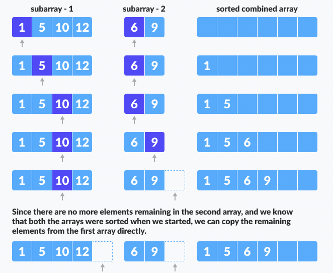
def merge_list(list1, list2): 
    list3 = []
    i = 0
    j = 0
  
    # Traverse both lists
    # If the current element of first list
    # is smaller than the current element
    # of the second list, then store the
    # first list's value and increment the index 

    while i < len(list1) and j < len(list2): 
      
        if list1[i] < list2[j]: 
            list3.append(list1[i])
            i += i
        else: 
            list3.append(list2[j])
            j += j
      
  
    # Store remaining elements of the first list
    while i < len(list1): 
        list3.append(list1[i])
        i += 1
  
    # Store remaining elements of the second list
    while j < len(list2): 
        list3.append(list2[j])
        j += 1
        
     #return list3 + list1[i:] + list2[j:]

    return list3

Time Complexity

• if n=8, $2^3 =8$, We will have 3 steps, so that log n.

• n: We will have insertion sort, so that nlog n.

• Best Case Complexity: O(nlog n)
• Worst Case Complexity: O(nlog n)
• Average Case Complexity: O(nlog n)

Space Complexity

• The space complexity of the merge sort is O(n).

Quick sort

• 기준 데이터를 설정하고 그 기준보다 큰 데이터와 작은 데이터의 위치를 바꾸는 방법이다.
• 일반적인 상황에서 가장 많이 사용되는 정렬 알고리즘 중 하나이다.
• 병합 정렬과 더불어 대부분의 프로그래밍 언어의 정렬 라이브러리의 근간이 되는 알고리즘이다.
• 가장 기본적인 퀵 정렬은 첫 번째 데이터를 기준 데이터(pivot)로 설정한다.

Quicksort is a sorting algorithm based on the divide and conquer approach where

1. An array is divided into subarrays by selecting a pivot element (element selected from the array).

   While dividing the array, the pivot element should be positioned in such a way that elements less than the pivot are kept on the left side, and elements greater than the pivot are on the right side of the pivot.

2. The left and right subarrays are also divided using the same approach. This process continues until each subarray contains a single element.

3. At this point, elements are already sorted. Finally, elements are combined to form a sorted array.

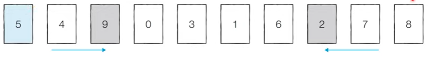
Working on Quicksort

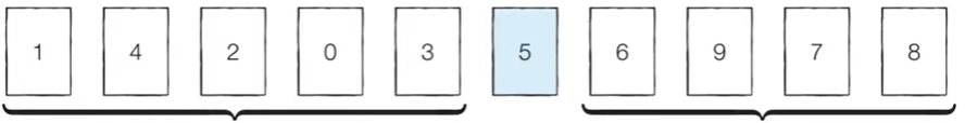
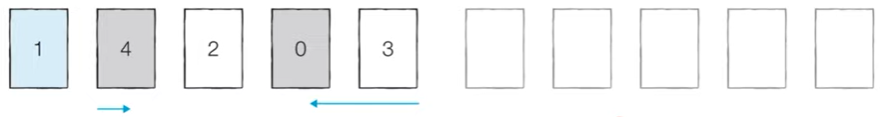
[Step 0] 현재 피벗의 값은 ‘5’이다. 왼쪽에서부터 ‘5’보다 큰 데이터를 선택하므로 ‘7’이 선택되고, 오른쪽에서부터 ‘5’보다 작은 데이터를 선택하므로 ‘4’가 선택된다.

[Step 1] 현재 피벗의 값은 ‘5’이다. 왼쪽에서부터 ‘5’보다 큰 데이터를 선택하므로 ‘9’가 선택되고, 오른쪽에서부터 ‘5’보다 작은 데이터를 선택하므로 ‘2’가 선택된다. 이제 이 두 데이터의 위치를 서로 변경한다.

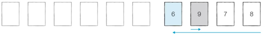
[Step 2] 현재 피벗의 값은 ‘5’이다. 왼쪽에서부터 ‘5’보다 큰 데이터를 선택하므로 ‘6’이 선택되고, 오른쪽에서부터 ‘5’보다 작은 데이터를 선택하므로 ‘1’이 선택된다. 단, 이처럼 위치가 엇갈리는 경우 ‘피벗’과 작은 데이터의 위치를 서로 변경한다.

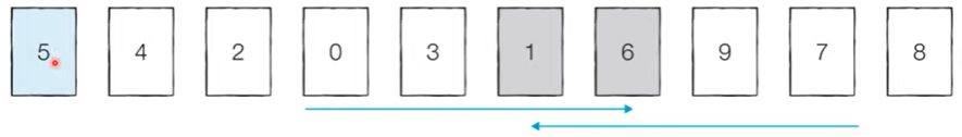
[분할 완료] 이제 ‘5’의 왼쪽에 있는 데이터는 모두 5보다 작고, 오른쪽에 있는 데이터는 모두 ‘5’보다 크다는 특징이 있다. 이렇게 피벗을 기준으로 데이터 묶음을 나누는 작업을 분할(Divide)이라고 한다.

[왼쪽 데이터 묶음 정렬] 왼쪽에 있는 데이터에 대해서 마찬가지로 정렬을 수행한다.

[오른쪽 데이터 묶음 정렬] 오른쪽에 있는 데이터에 대해서 마찬가지로 정렬을 수행한다. 이러한 과정을 반복하면 전체 데이터에 대해서 정렬이 수행된다.

Why is it so quick?

• 이상적인 경우 분할이 절반씩 일어난다면 전체 연산 횟수로 $O(NlogN)$를 기대할 수 있다. 너비 X 높이 = N X logN = NlogN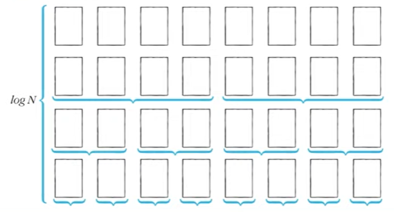

Source code 1

array = [5,7,9,0,3,1,6,2,4,8]

def quick_sort(array, start, end):
	if start >= end:  # 원소가 1개인 경우 종료
    	return
  pivot = start  # 피벗은 첫 번째 원소
  left = start + 1
  right = end
  while(left <= right): #선형 탐색
    	# 피벗보다 큰 데이터를 찾을 때까지 반복
      while(left <= end and array[left] <= array[pivot]):
      	left += 1
        # 피벗보다 작은 데이터를 찾을 때까지 반복
      while(right>start and array[tight]>=array[pivot]):
      	right -= 1
      if(left>right):  # 엇갈렸다면 작은 데이터와 피벗을 교체
      	array[right], array[pivot] = array[pivot], array[right]
		  else:  # 엇갈리지 않았다면 작은 데이터와 큰 데이터를 교체
        	array[left], array[right] = array[right], array[left]
    # 분할 이후 왼쪽 부분과 오른쪽 부분에서 각각 정렬 수행
  quick_sort(array, start, right-1)
  quick_sort(array, right+1, end)

quick_sort(array, 0, len(array)-1)
print(array)

#[실행 결과]
[0,1,2,3,4,5,6,7,8,9]

Source code 2 (Easier with Python)

#List Comprehension을 이용하여 더 간결하게!
array = [5,7,9,0,3,1,6,2,4,8]

def quick_sort(array):
	# 리스트가 하나 이하의 원소만을 담고 있다면 종료
    if len(array) <= 1:
    	return array
    pivot = array[0]  # 피벗은 첫 번째 원소
    tail = array[1:]  # 피벗을 제외한 리스트
    
    left_side = [x for x in tail if x <= pivot]  # 분할된 왼쪽 부분
    right_side = [x for x in tail if x > pivot]  # 분할된 오른쪽 부분
    
    # 분할 이후 왼쪽 부분과 오른쪽 부분에서 각각 정렬 수행하고, 전체 리스트 반환
    return quick_sort(left_side) + [pivot] + quick_sort(right_side)
    
print(quick_sort(array))

Time Complexity

• 퀵 정렬은 평균의 경우 $O(N\log N)$의 시간 복잡도를 가진다.
• 하지만 최악의 경우 $O(N^2)$의 시간 복잡도를 가진다. 첫 번째 원소를 피벗으로 삼을 때, 이미 정렬된 배열에 대해서 퀵 정렬을 수행할 경우 최악의 경우이다.
  • 
• 표준 라이브러리를 사용하는 경우, 기본적으로$O(N\log N)$을 보장한다.

Counting Sort (계수 정렬)

• 특정한 조건이 부합할 때만 사용할 수 있지만 매우 빠르게 동작하는 정렬 알고리즘이다. 계수 정렬은 데이터의 크기 범위가 제한되어 정수 형태로 표현할 수 있을 때 사용 가능하다.
• 데이터의 개수가 N, 데이터(양수) 중 최댓값이 K일 때 최악의 경우에도 수행시간 $O(N+K)$를 보장한다.

Working on Counting Sort

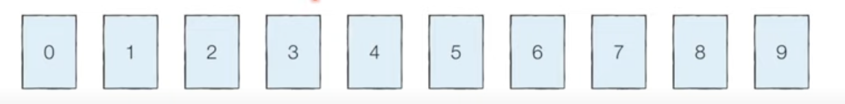
[Step 0] 가장 작은 데이터로부터 가장 큰 데이터까지의 범위가 모두 담길 수 있도록 리스트를 생성한다.

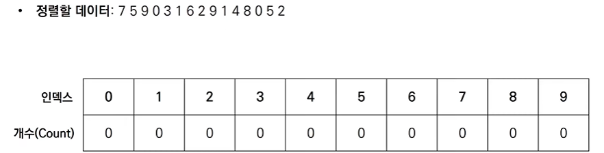
인덱스는 0~9의 숫자로 구성된 것을 확인할 수 있고, 이때 각 인덱스가 데이터의 값에 해당한다.

[Step 1] 데이터를 하나씩 확인하며 데이터의 값과 동일한 인덱스의 데이터를 1씩 증가시킨다.

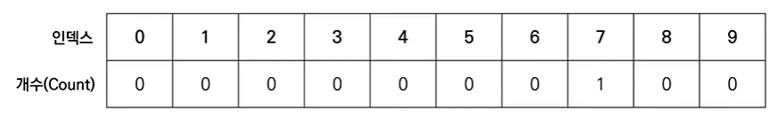
[Step 2] 데이터를 하나씩 확인하며 데이터의 값과 동일한 인덱스의 데이터를 1씩 증가시킨다.

결과적으로 최종 리스트에는 각 데이터가 몇 번씩 등장했는지 그 횟수가 기록된다.

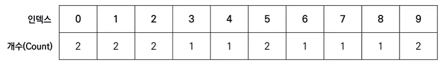
결과를 확인할 때는 리스트의 첫 번째 데이터부터 하나씩 그 값만큼 반복하여 인덱스를 출력한다.

[출력 결과] 001122345567899 각각의 데이터가 몇번씩 등장했는지 세는 방식으로 동작하는 정렬 알고리즘이다.

Source code

# 모든 원소의 값이 0보다 크거나 같다고 가정
array = [7,5,9,0,3,1,6,2,9,1,4,8,0,5,2]

# 모든 범위를 포함하는 리스트 선언(모든 값은 0으로 초기화)
count = [0]*(max(array)+1)

for i in range(len(array)):
	count[array[i]] += 1  # 각 데이터에 해당하는 인덱스의 값 증가: O(N)

for i in range(len(count)):  # 리스트에 기록된 정렬 정보 확인: O(K)
	for j in range(count[i]):
    	print(i, end=' ')  # 띄어쓰기를 구분으로 등장한 횟수만큼 인덱스 출력
#0 0 1 1 2 2 3 4 5 5 6 7 8 9 9

Time Complexity

• 계수 정렬의 시간 복잡도와 공간 복잡도는 모두 O(N+K)이다.
• 계수 정렬은 때에 따라서 심각한 비효율성을 초래할 수 있다. 데이터가 0과 999,999로 단 2개만 존재하는 경우, 백만개 만큼의 원소가 담길 수 있는 배열을 만들어야 한다.
• 계수 정렬은 동일한 값을 가지는 데이터가 여러 개 등장할 때 효과적으로 사용할 수 있다.
  • 성적의 경우 100점을 맞은 학생이 여러 명일 수 있기 때문에 계수 정렬이 효과적.

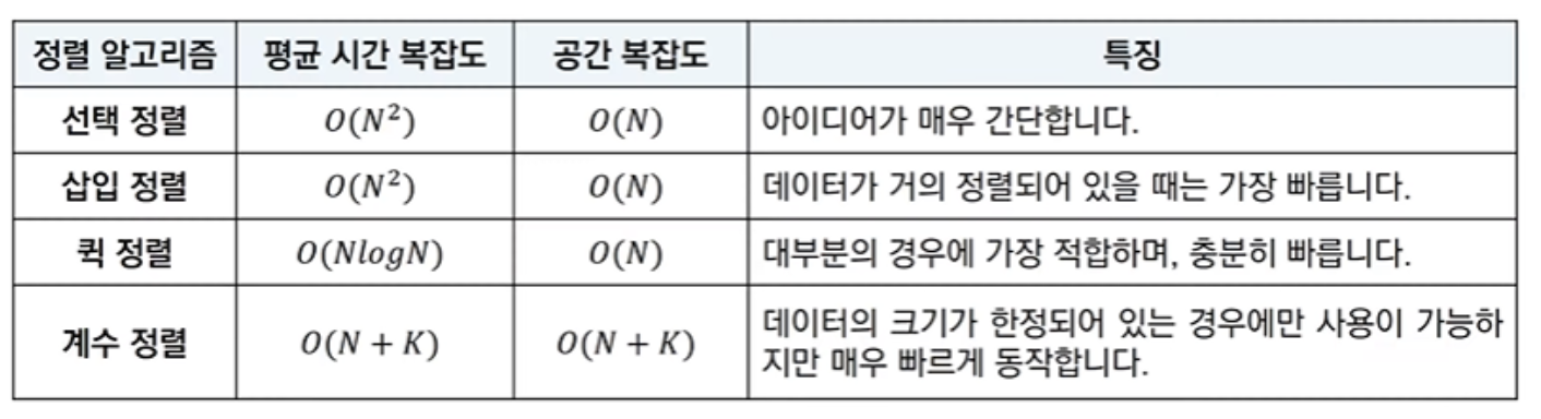
Comparison of Sorting Algorithms

• 추가적으로 대부분의 프로그래밍 언어에서 지원하는 표준 정렬 라이브러리는 최악의 경우에도 $O(N\log N)$을 보장하도록 설계되어 있다.
• 퀵 정렬의 경우, 구현 방식에 따라 최악의 경우 시간 복잡도가 O(N^2)$이 나올 수 있다.

Comparison of Time

from random import randint 
import time

# 배열에 10,000개의 정수를 삽입
array = []
for _ in range(10000):
	# 1부터 100 사이의 랜덤한 정수
    array.append(randint(1,100))
    
# 선택 정렬 프로그램 성능 측정
start_time = time.time()

# 선택 정렬 프로그램 소스코드
for i in range(len(array)):
	min_index = i  # 가장 작은 원소의 인덱스
    for j in range(i+1, len(array)):
    	if array[min_index] > array[j]:
        	min_index = j
    array[i], array[min_index] = array[min_index], array[i]
    
# 측정 종료
end_time = time.time()
# 수행 시간 출력
print("선택 정렬 성능 측정:", end_time - start_time)

# 배열을 다시 무작위 데이터로 초기화
array = []
for _ in range(10000):
	# 1부터 100 사이의 랜덤한 정수
    array.append(randint(1,100))

# 기본 정렬 라이브러리 성능 측정
start_time = time.time()

# 기본 정렬 라이브러리 사용
array.sort()

# 측정 종료
end_time = time.time()
print("기본 정렬 라이브러리 성능 측정:", end_time - start_time)
#[실행 결과]
#선택 정렬 성능 측정: 35.841460943222046
#기본 정렬 라이브러리 성능 측정: 0.0013387203216552734

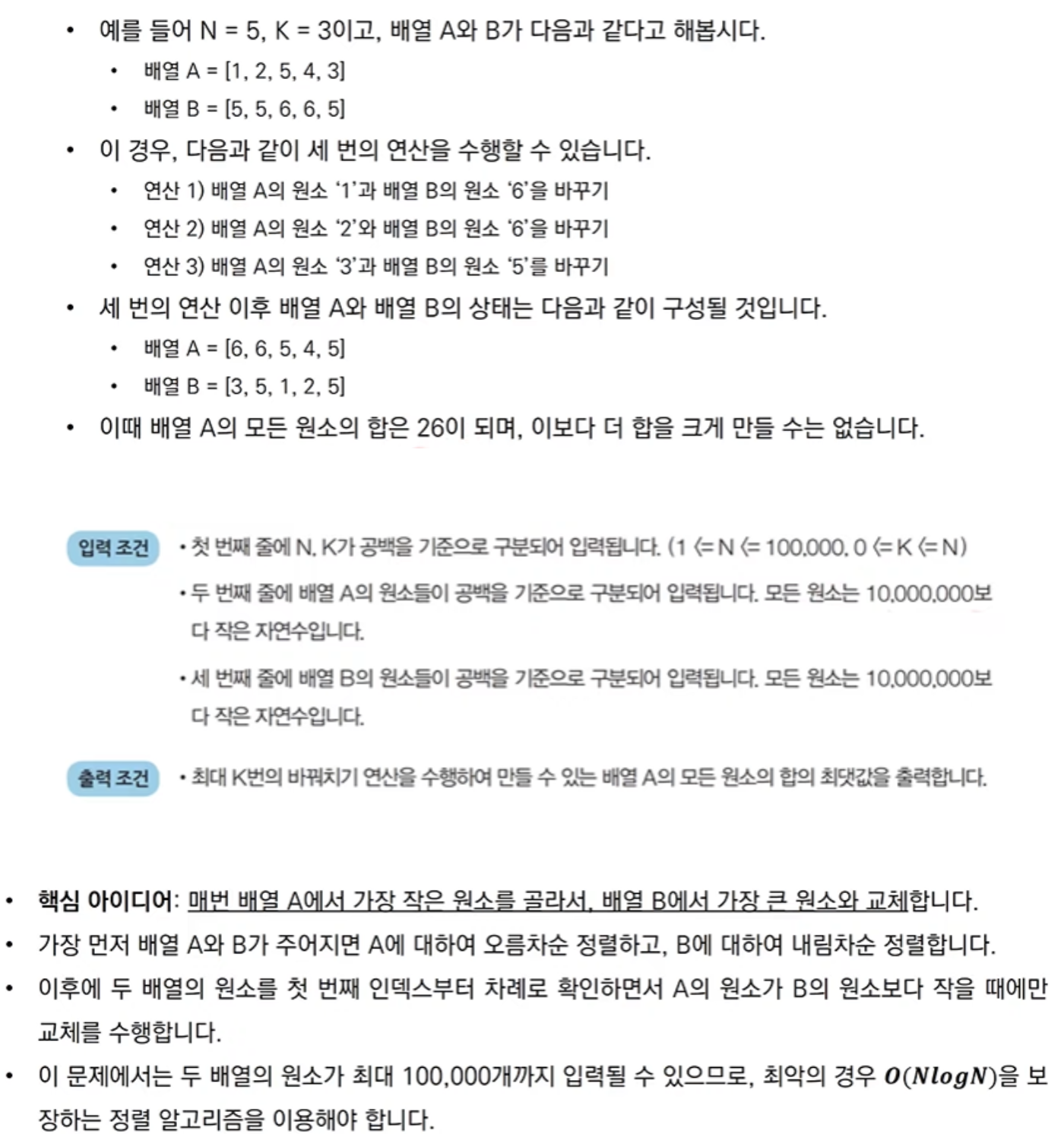
Example 1: 두 배열의 원소 교체

• 동빈이는 두 개의 배열 A와 B를 가지고 있습니다. 두 배열은 N개의 원소로 구성되어 있으며, 배열의 원소는 모두 자연수입니다.
• 동빈이는 최대 K번의 바꿔치기 연산을 수행할 수 있는데, 바꿔치기 연산이란 배열 A에 있는 원소 하나와 배열 B에 있는 원소 하나를 골라서 두 원소를 서로 바꾸는 것을 말합니다.
• 동빈이의 최종 목표는 배열 A의 모든 원소의 합이 최대가 되도록 하는 것이며, 여러분은 동빈이를 도와야 합니다.
• N, K 그리고 배열 A와 B의 정보가 주어졌을 떄, 최대 K번의 바꿔치기 연산을 수행하여 만들 수 있는 배열 A의 모든 원소의 합의 최댓값을 출력하는 프로그램을 작성하세요.

n, k = map(int, input().split())  # N과 K를 입력 받기
a = list(map(int, input().split()))  # 배열 A의 모든 원소를 입력 받기
b = list(map(int, input().split()))  # 배열 B의 모든 원소를 입력 받기

a.sort()  # 배열 A는 오름차순 정렬 수행
b.sort(reverse=True)  # 배열 B는 내림차순 정렬 수행

# 첫 번째 인덱스부터 확인하며, 두 배열의 원소를 최대 K번 비교
for i in range(k):
	# A의 원소가 B의 원소보다 작은 경우
    if a[i] < b[i]:
    	# 두 원소를 교체
        a[i], b[i] = b[i], a[i]
    else:
    	break

print(sum(a))  # 배열 A의 모든 원소의 합을 출력